RNN Learning

[toc]

Vanilla RNN Architecture

Abstract design

RNN is the abbreviation of the Recurrent Neural Network. A piece of slice in RNN (because it is recurrent) is as below:

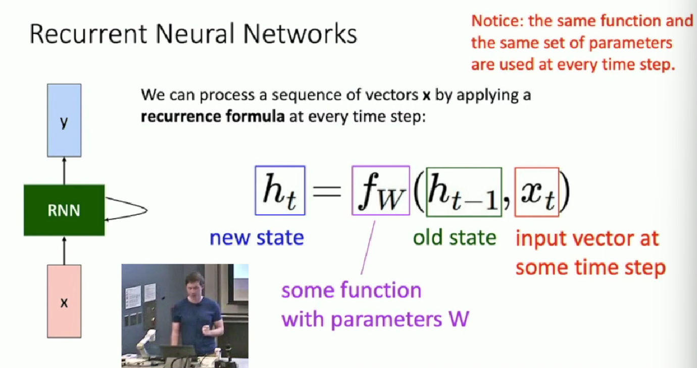
For each iteration, a piece of RNN model receives a current input (optional), and combine it with the previous state to send to the processing function (linear weight and non-linear activation function) to produce the new state. The new state can then used to generate the current output (optional). The hidden transition of state is important!

Notice: the same function and the same set of parameters are used at every time step.

Concrete implementation

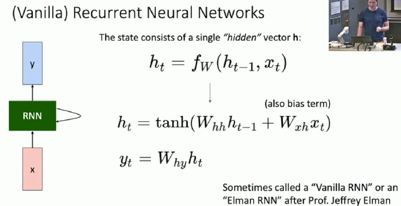
In this implementation we need to train $W_{hh}$ and $W_{xh}$ in the end

Composed computation graph

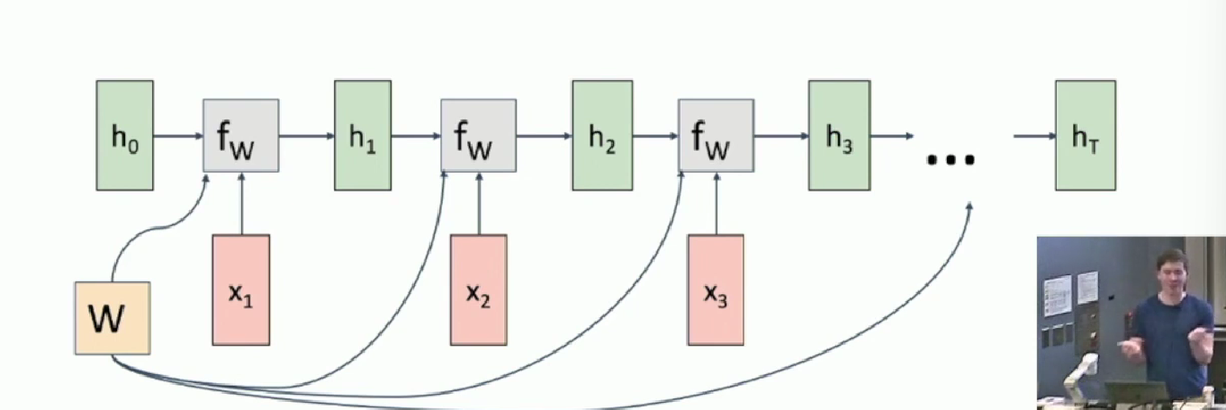
As the node is copied many times, the backpropagation result of each node should be sum up to update W.

For different usage, the output and loss function may varies.

A typical one is as following:

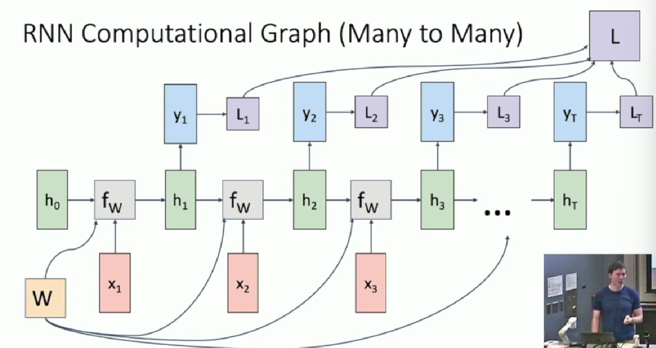
Others includes one-to-many, many-to-one, seq-to-seq. Not listed here

Example: Language Modeling

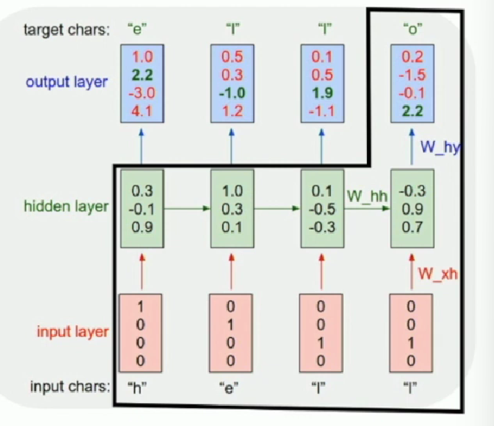
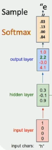
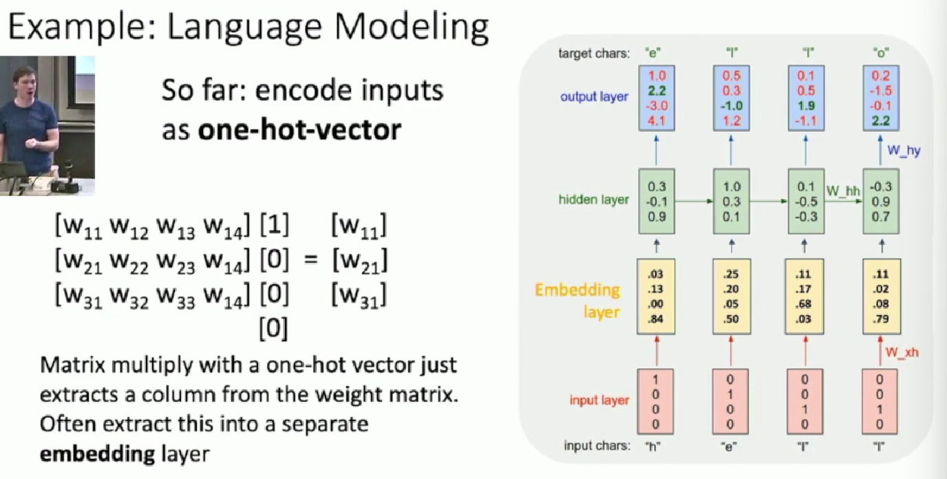
Notice that one-hot-vector matmul is just extracting one col in the weight matrix, so we can also create an embedding layer that helps do the extraction job

Truncated Backprop

To save memory, we can use truncated backprop, where we do forward prop for the whole model sequence, but we only backprop within every truncated chunk of model. This is done by first truncate the model, then at each disconnected area, we calculate the current loss and pass current (output, hidden state) to the next chunk as (input, hidden state). Because the input is sent forth, the loss calculation will be continuous or global in the process. But we do not receive the upstream gradient to compute local gradient. Instead, we use the loss function that we calculate locally and do backpropagation within the chunk respectively, and update weight.

Vanilla RNN in Image Captioning

As a concrete example, we want to output a description of a given input image. What will the model structure be like?

The model can be a combination of CNN and RNN, where CNN provide the understanding of picture information, and RNN is responsible for sentence generation. A simplified architecture is given below:

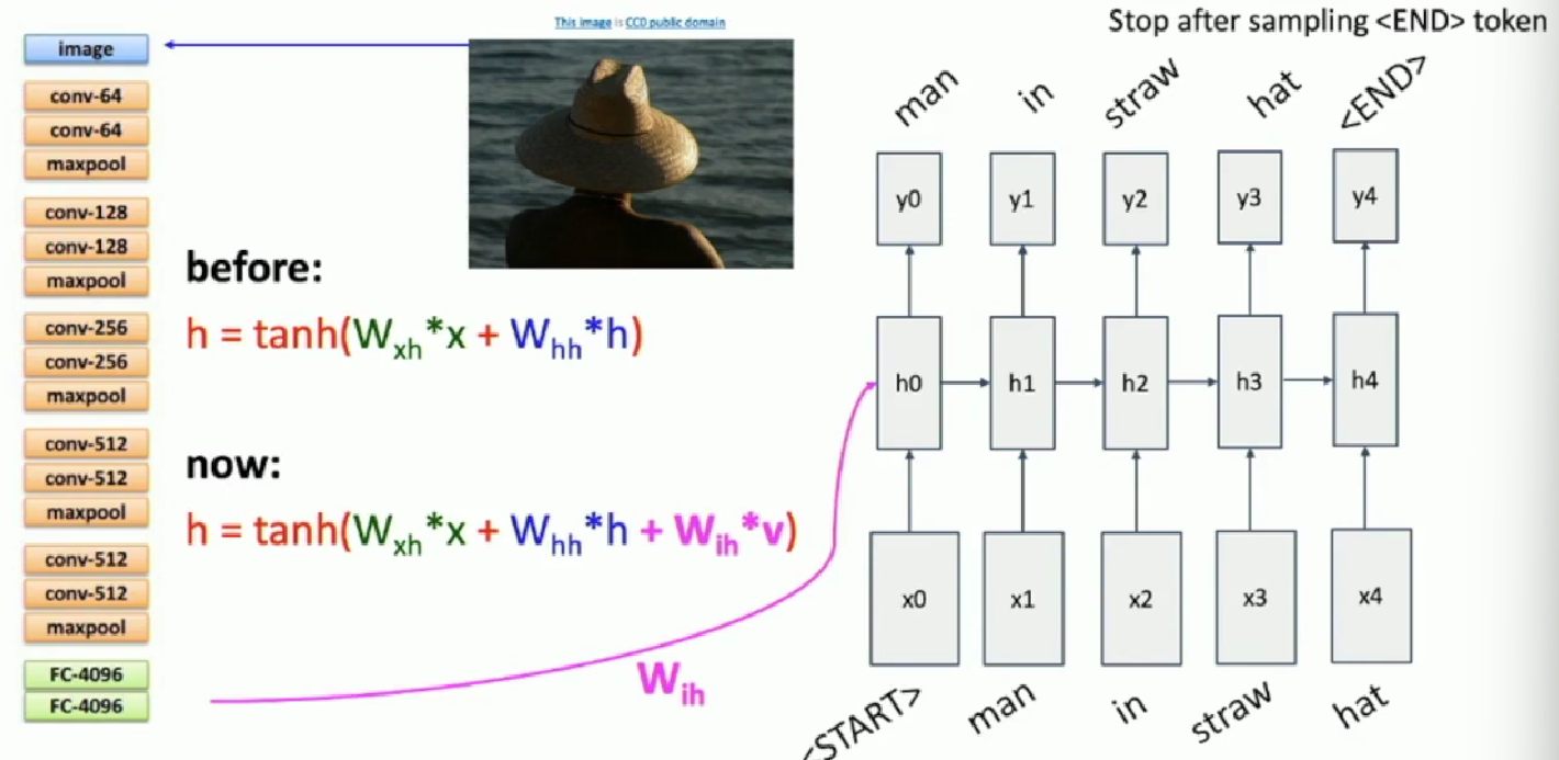Notice that our RNN model will receive another image input from CNN so as to understand the picture. Also <start> and <end> token (the term “token” is the single output for a single slice of RNN) will be used to control the model, namely when the model predicts a <stop> token, the model stop generating sentences.

Drawbacks

Vanilla RNN had a hard time in conducting weight propagation.

By chain rule, the longer an RNN is, the more node it will pass for those nodes at the beginning of RNN. And as they share the same update rules, for example, dXH_stacked = torch.matmul(dtanh * W.transpose() ) . By chain rule, when multiply them for many times, as long as W has a singular value that > 1 or < 1, by propagation, the gradient will correspondently explode or vanish, and leads to failure in gradient descend afterwards.

Here is the map of a computational graph for vanilla RNN.

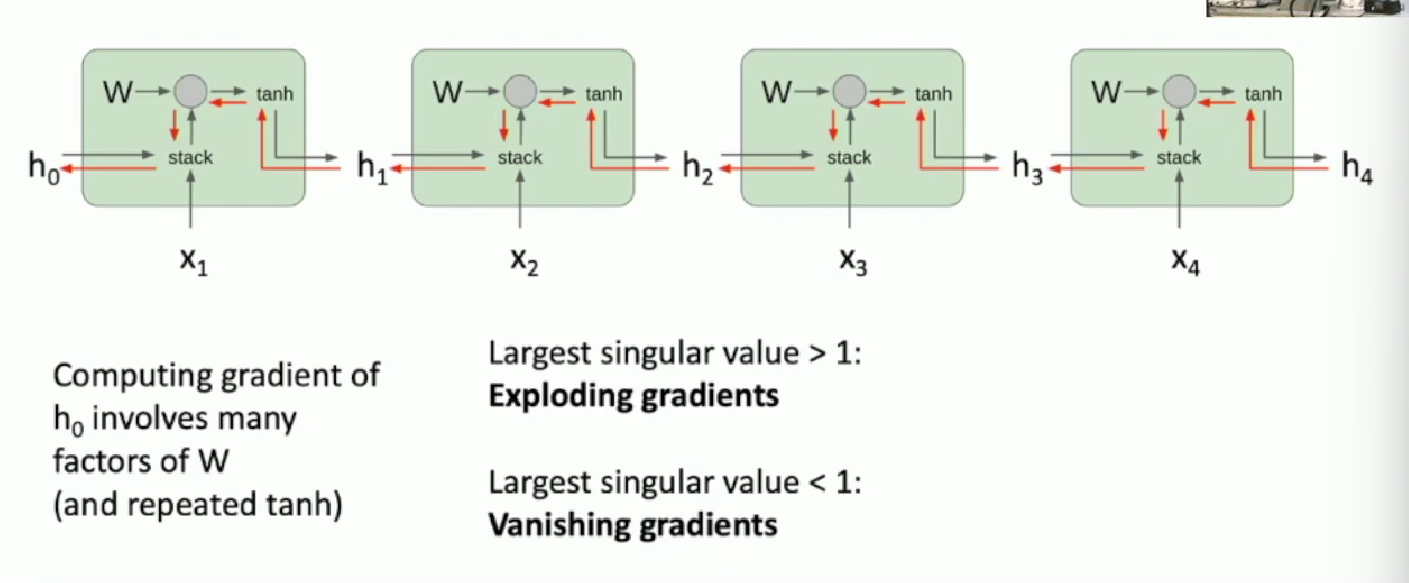
The red roadmap is the only way the upstream gradient can affect the successive gradients. And with its update rule is listed above, the gradient vanish & explode problem is clear to be justified.

LSTM

Abstract design

It turns out that RNNs can have various update functions, and many times the update function is the only main difference between two RNN architectures. It turns out LSTM is one example.

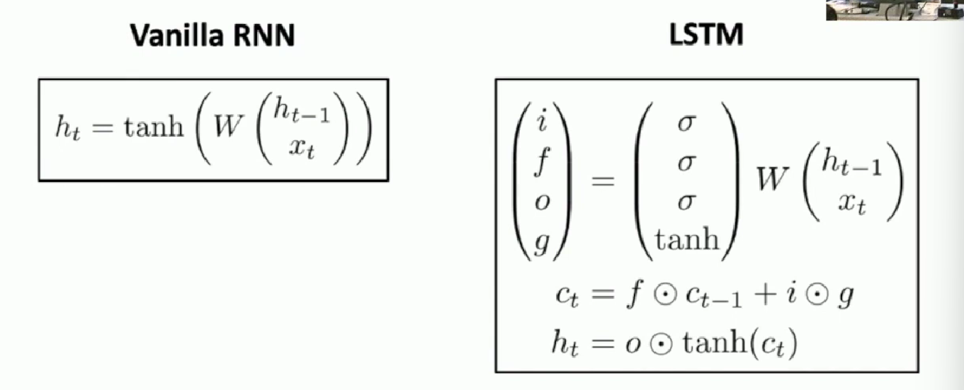
The update rules of LSTM seems complicated in this way. A visualized computational graph may be helpful.

The above formula tells the following things.

The first equation should be read from right to left. We first stack previous hidden state and the current input x , and compute through a weight matrix. Then we divide the output vector into four piece and sent to sigmoid or tanh function, the output will be four gate units which serves as temporal local variables in one slice of LSTM. Somehow they have names and particular meanings to be interpreted.
The second line computes a new remembered status for LSTM: $c_t$ , the cell status.
The third computes update of the commonly remembered status: the hidden state.
The output label and loss function is not include and can be tuned by the engineers.

Gate unit and its interpretation

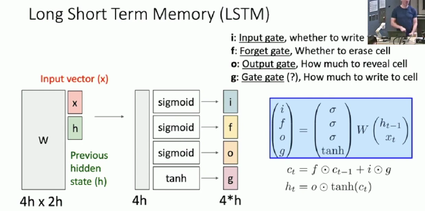
By looking at formular two and three, we see Input gate is determining what to write to the cell status
Forget gates controls how many information is going to be communicated between the two adjacent layers.
Output gate controls how much will the cell status be revealed as hidden layer, and further be calculated in this output.
Gate/Control gate controls how much will the input gate information be written into the cell status. Notice that it is the only gate unit that has negative output. which corresponds to showing negative contribution.

Computational Graph

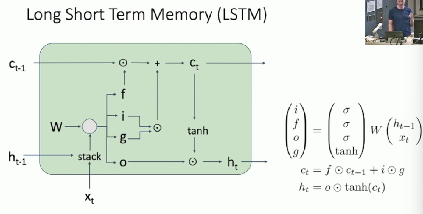
The above is the single sliced LSTM model. Cascaded version is as below

The perspective is that at least there is one way that is friendly for upstream gradient to go down without much duplicating calculation that cause gradient explode or vanishing.

Multiplayer RNNs

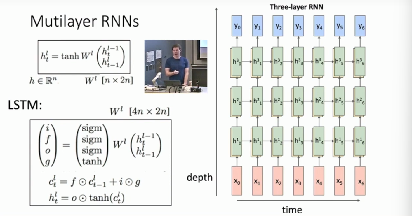
Without surprise, RNNs can be stacked together and go deeper in another dimension except the time axis.

When stacked, the output hidden state not only becomes the input of the next node’s input along time axis, but also is the input of the next node along the depth dimension. Here is the visualization.

GRU and other RNN variants

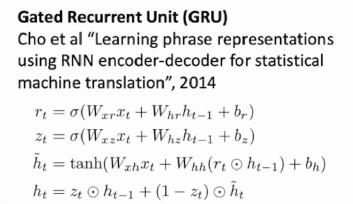
As have said before, many RNN architectures differ only mainly in their update functions. GRU and LSTM is one of them. The update function of GRU is as following: