Attention Learning

Attention Mechanism Learning Notes

Fundamentals for Attention Mechanism

Vanilla Seq2seq RNNs

In previous lecture, we talk about seq2seq RNN model.

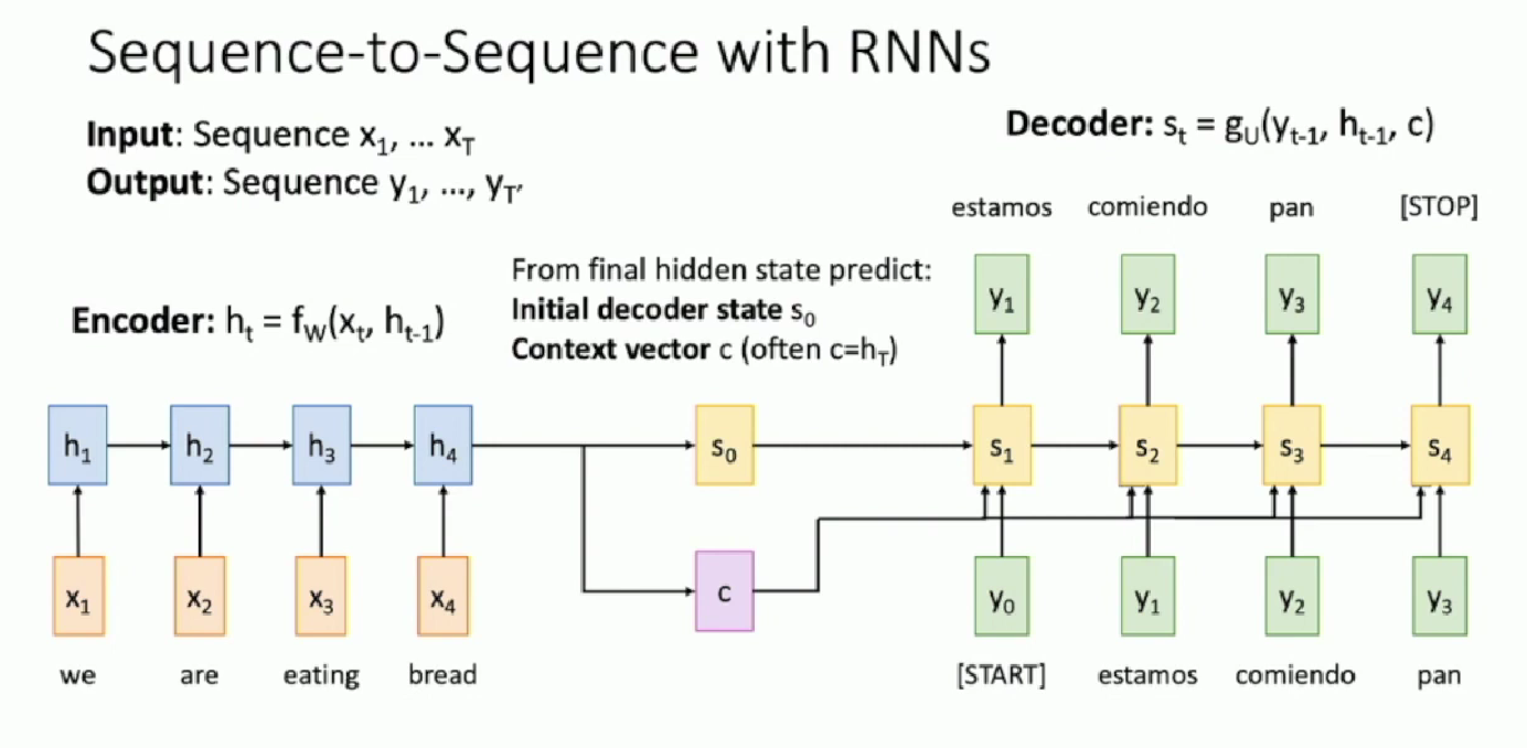
Specifically, the vanilla version is to transform the output hidden state from the encoder model into two part ($s_0$ and $c$ ) and then send them to the input side of the decoder model.

Typically, the decoder will use $c$ as a context vector and view it as having stored all the information of the encoder model. Thus $c$ is going to be one of the input of all the sliced decoder henceforth. On the other hand $s_0$ will be viewed as the previous hidden state for the decoder RNN. $s_0$ is usually set to zero, and $c$ is usually set to hout.T

Seq2seq with Attention Mechanism

To avoid use a single context vector, we want the context vector to be generated for each slice of decoder model through the time. The mechanism to do it is called the attention mechanism.

The principle of attention model is as following:

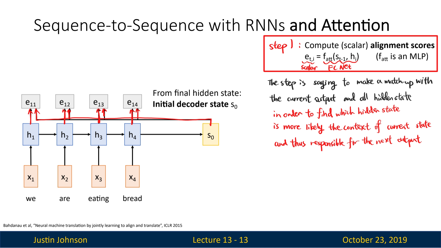
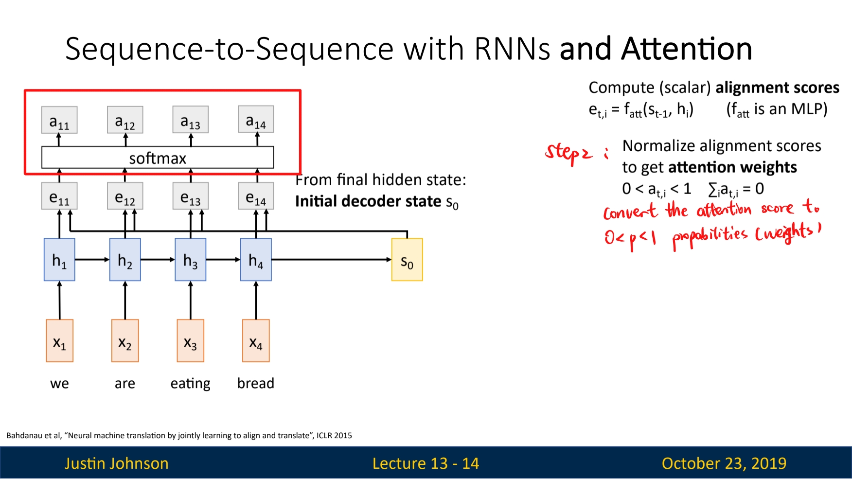
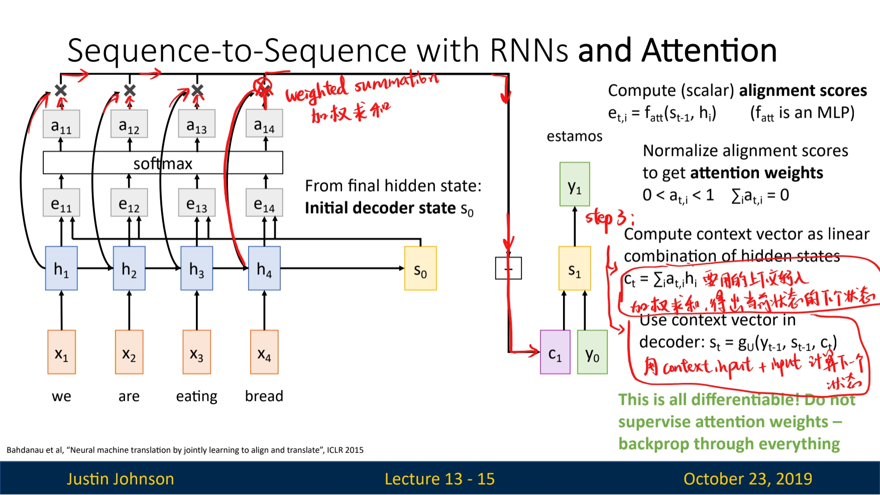
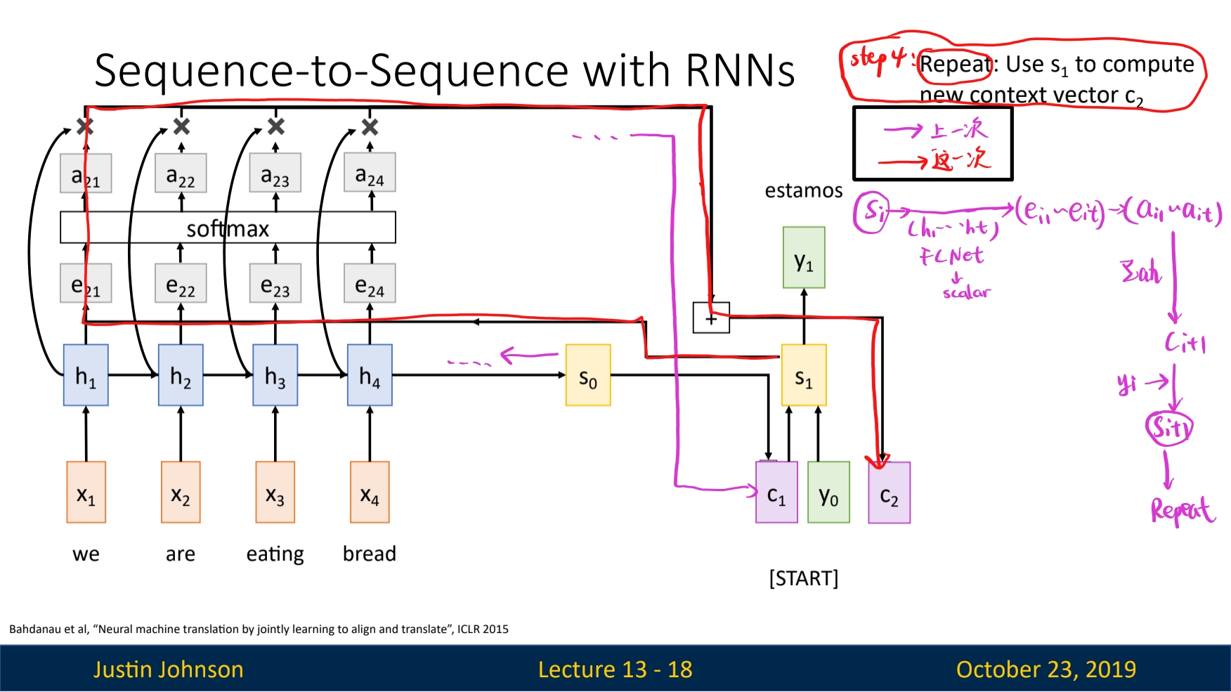
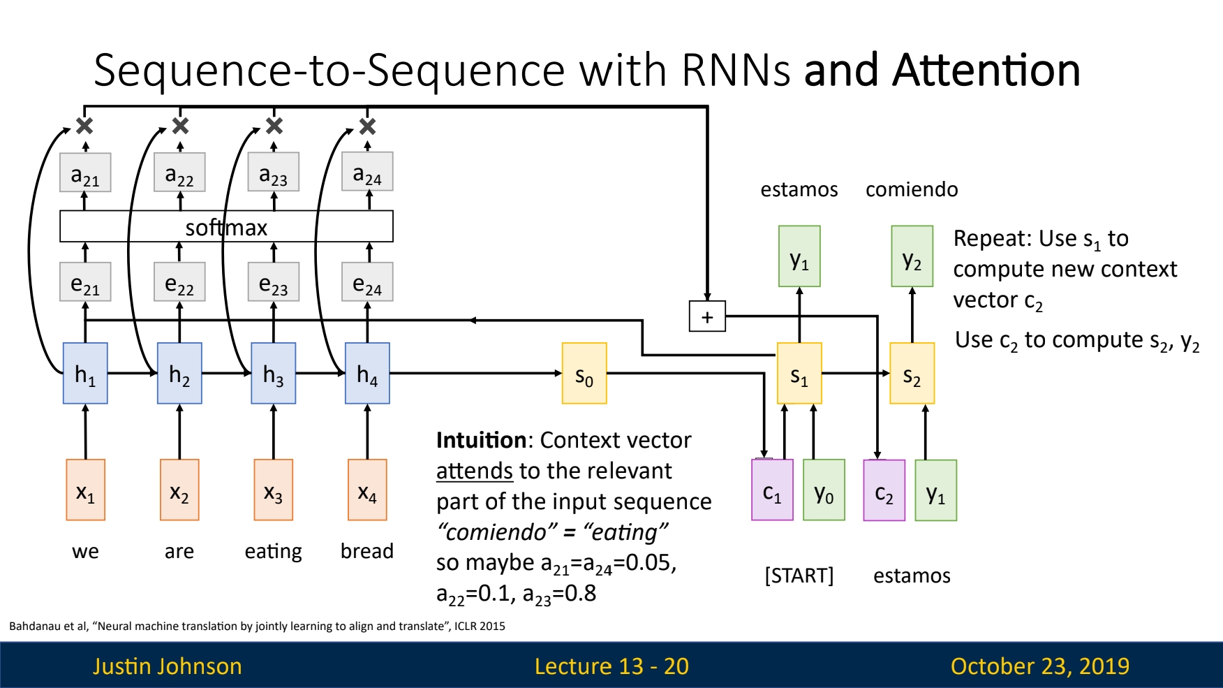
Correction: the result of the output of the FC layer in step 1, denoted as e also has a academic name, the alignment score. And the process of $s_i$ and $h$ be sent to a FC net like function $f_{att}$ is called the alignment operation.

Image Captioning with RNNs and Attention

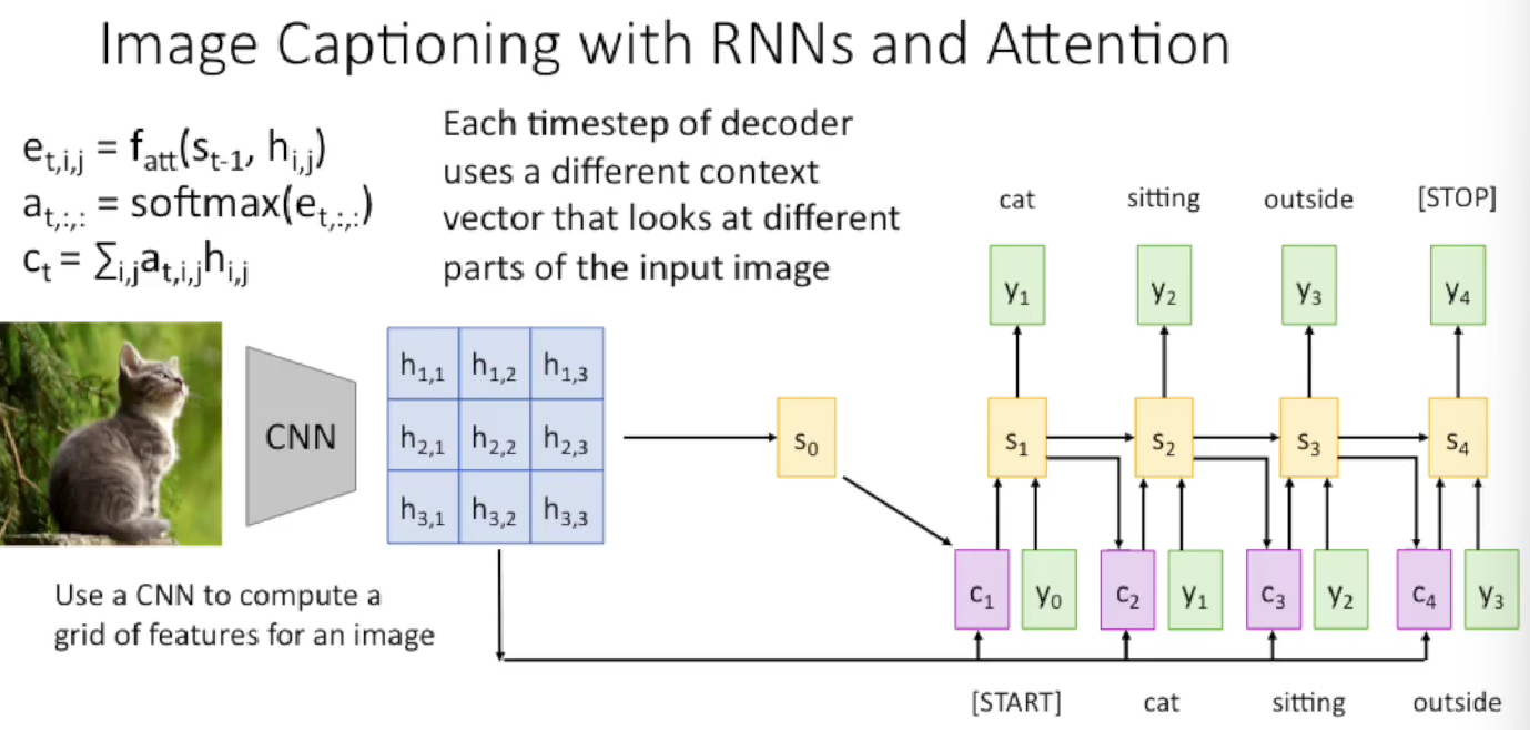
In this example it is meaningful to look at the shape of the computation.

• The feature grid $[h_{ij}]$ is an output of one layer in the Convolutional Network. So the $h_{ij}$ is a vector with length equals to the depth of features (the number of kernels of the current conv layer, and in all the shape after one conv should be CxHxW, C is the kernel number of this layer). We don’t consider batch here currently.
• $e_{tij}$ is a scalar, and so does $a_{tij}$ , which is the attention score/prop of the feature vector $h_{ij}$ at location (i,j) on the feature grid.
• $c_t$ is a vector, a linear combination or weighted sum of vector $h_{ij}$ .
• $s_t$ is a vector, but is the hidden state affiliated to RNN structure. The hidden state is always a vector.

Attention Layer

Abstraction into Signs

Given that we can apply attention mechanism to lots of applications, we tend to wrap it up, and make abstractions on it independently so that it can be encapsulated into more applications.

The first thing we need to the is use signature language to express the problem.

The following is the first abstraction.

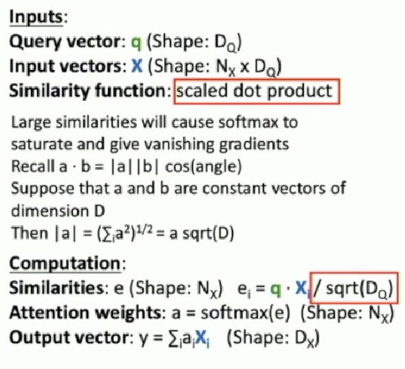
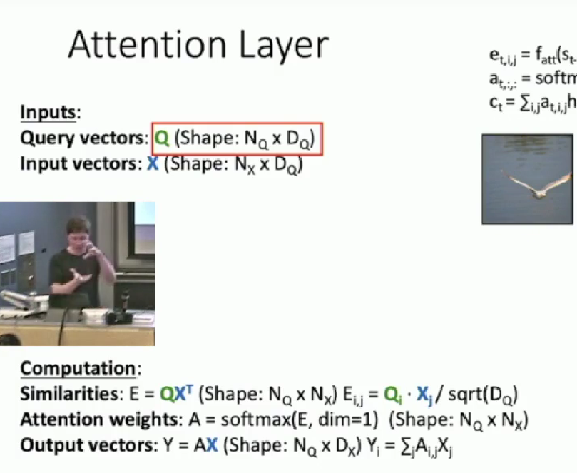
Remember that in previous examples, we have a current hidden state in decoder and want to compare it with all the hidden states in the encoder. This process has been abstracted into following:

• The hidden state that initiate the attention process is called a query vector q. Given q is from RNN, it should be a vector of shape $D_Q$
• All the hidden state that the query vector q want to compare to is called the input vectors. Given if we have N number of X, we stack them together so that the shape is (N, $D_Q$)
• Before we do similarity comparison to all the X and the q, with function $f_{att}$. Now the function is replaced by scaled dot product , the computation is in the illustration above. Note that the scaled constant sqrt($D_Q$) comes from the idea of normalizing the vector better according to their number of dimension. High dimensional vectors tend to have bigger dot product, considering the geometric equation of the dot product.
• The Softmax and the Weighted sum operation remain the same

Extent to Multiply Queries

We now extent the query vector into query vectors. Meaning the query vectors should be a matrix, with each row representing a query. This extents the scaled dot product to scaled matrix multiplication and weighted sum to another matrix multiplication, finally the Softmax function should still be doing to each query, namely each row of the attention weight matrix A, so Softmax should be done with dim=1.

The detailed extension and shape expression are given as below:

Add Flexibilities

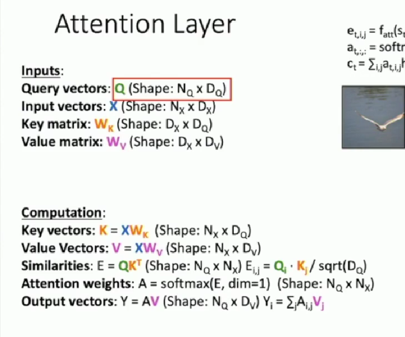
Notice that we use the input vectors twice, one in comparing similarity (attention scores), another in computing the output vectors.

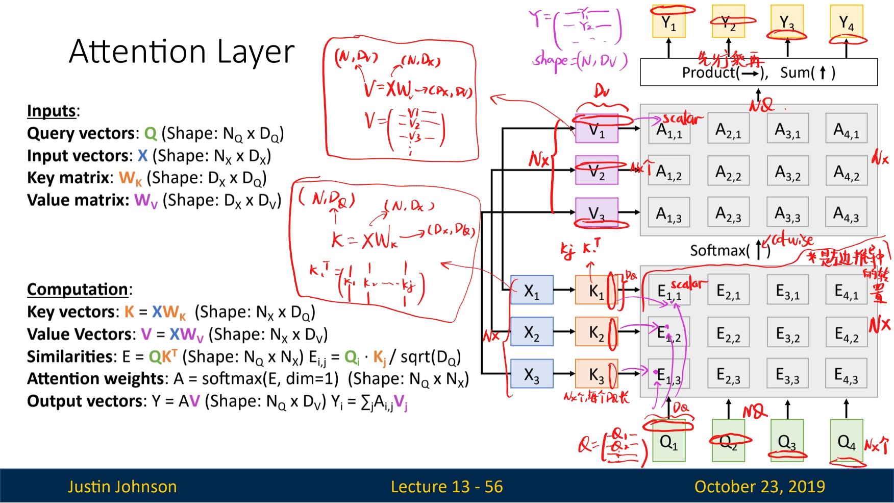
To add more flexibilities on the input vector, we transform the input vectors X into two types and then sent to two usages. Specifically, key matrix for similarity comparison, and value matrix for output computation. The details are shown in below

A clear computational graph may help a lot!

Become self-attention

Sometimes there are no queries as input. Instead we want to generate the queries from input vectors $X$, aka the hidden states. That requires another learnable weight matrix. The architecture is as following:

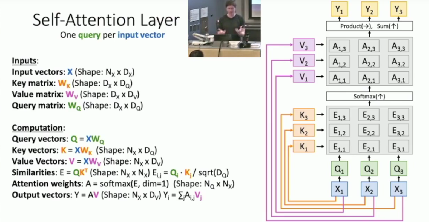
A common error: $N_Q$ and $N_x$ are different! They differ because Q is processed by multiplying $W_Q$ , previously they are also different, but that comes from queries being another input.

$N_Q$ and $N_x$ are different, which lead to the output Y with number $N_Q$ and the only input X with number $N_X$ having different numbers. Be careful!

More over, $N_Q$ now is a hyperparameter!

The computation is not affected by the permutation of input vectors $X$, the operations are still aligned. This is called the Permutation Equivariant . The following shows an example

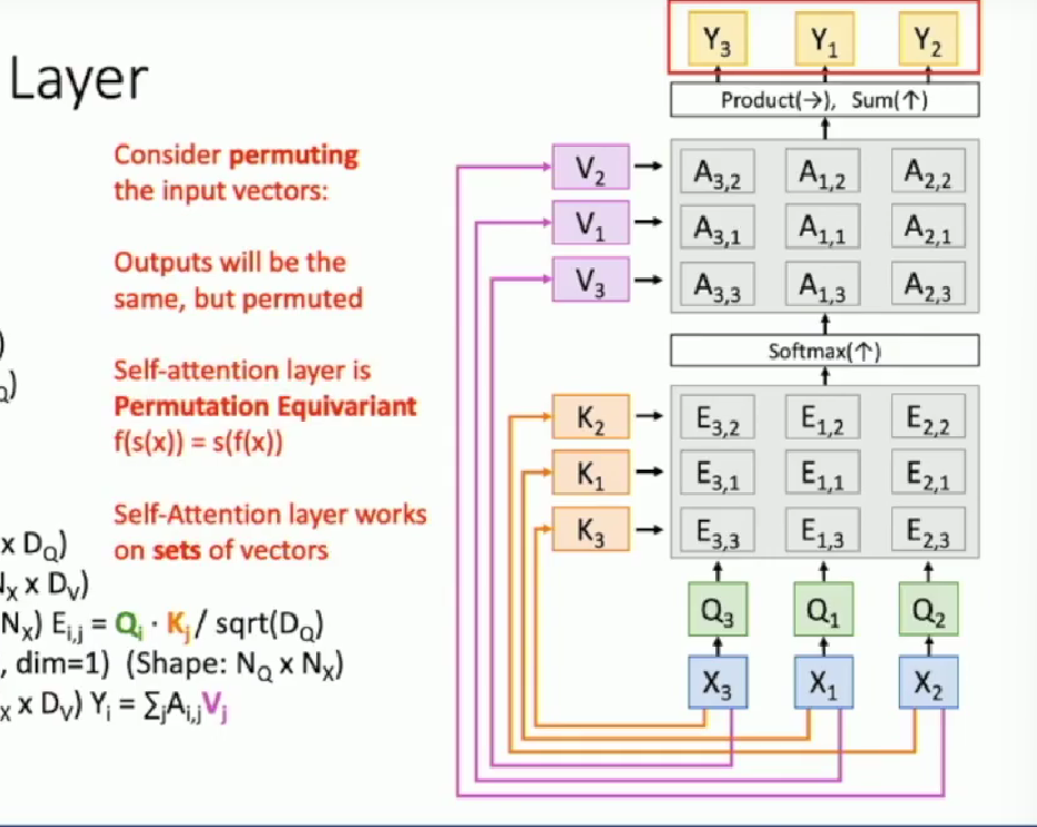
This can be a drawback! For example, we want the probability of the period (.) to be larger when sentence is long. So we need to add more information on locations to the input (of self-attention layer). One way of this is as the following:

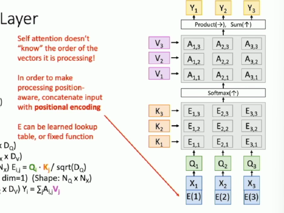
Variants of the Self-Attention Layer

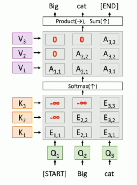
1. Masked self-attention layer

Some model requires casualty , the answer to the query should use only information hitherto, like for Q2 we only offer hidden state h1 and h2 (actually their key values K1, K2). A typical application may be translation, and audio understanding, where the input is time aligned from the physical world.

The computational graph is as following:

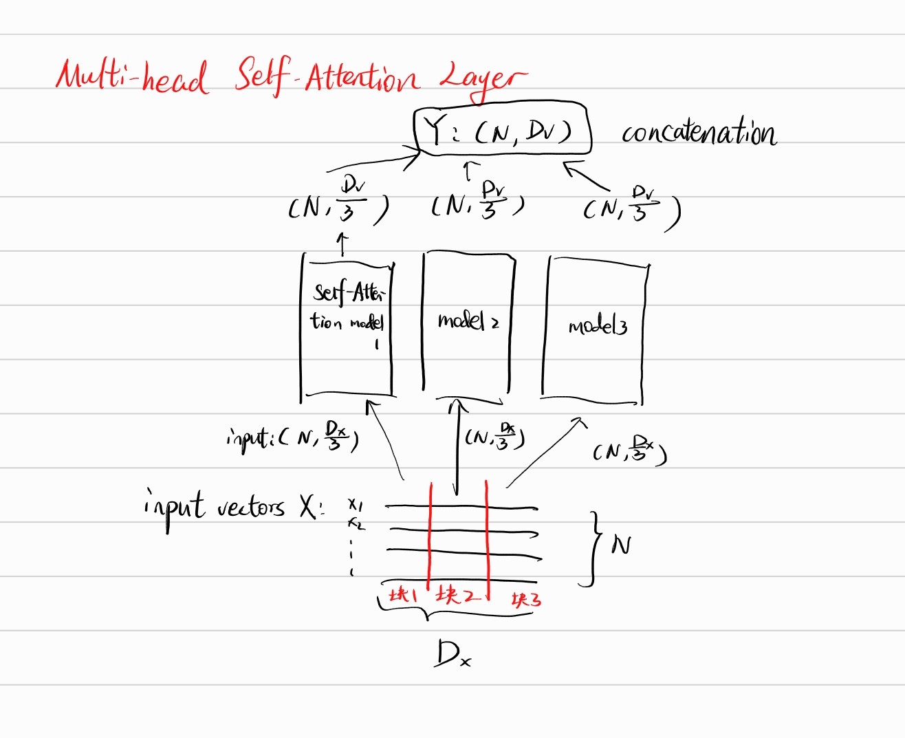
2. Multi-head self-attention

   Sometimes we see architectures that divide input in Dx dimension and sent each truncated input to parallel self-attention inputs. Then collect and concatenate the output to form the result matrix Y. The truncated number of chunks (number of heads) and the query dimension generated by input vectors X within each self-attention models are two hyperparameters that we want to tune.

   

Attention Model in ConvNet

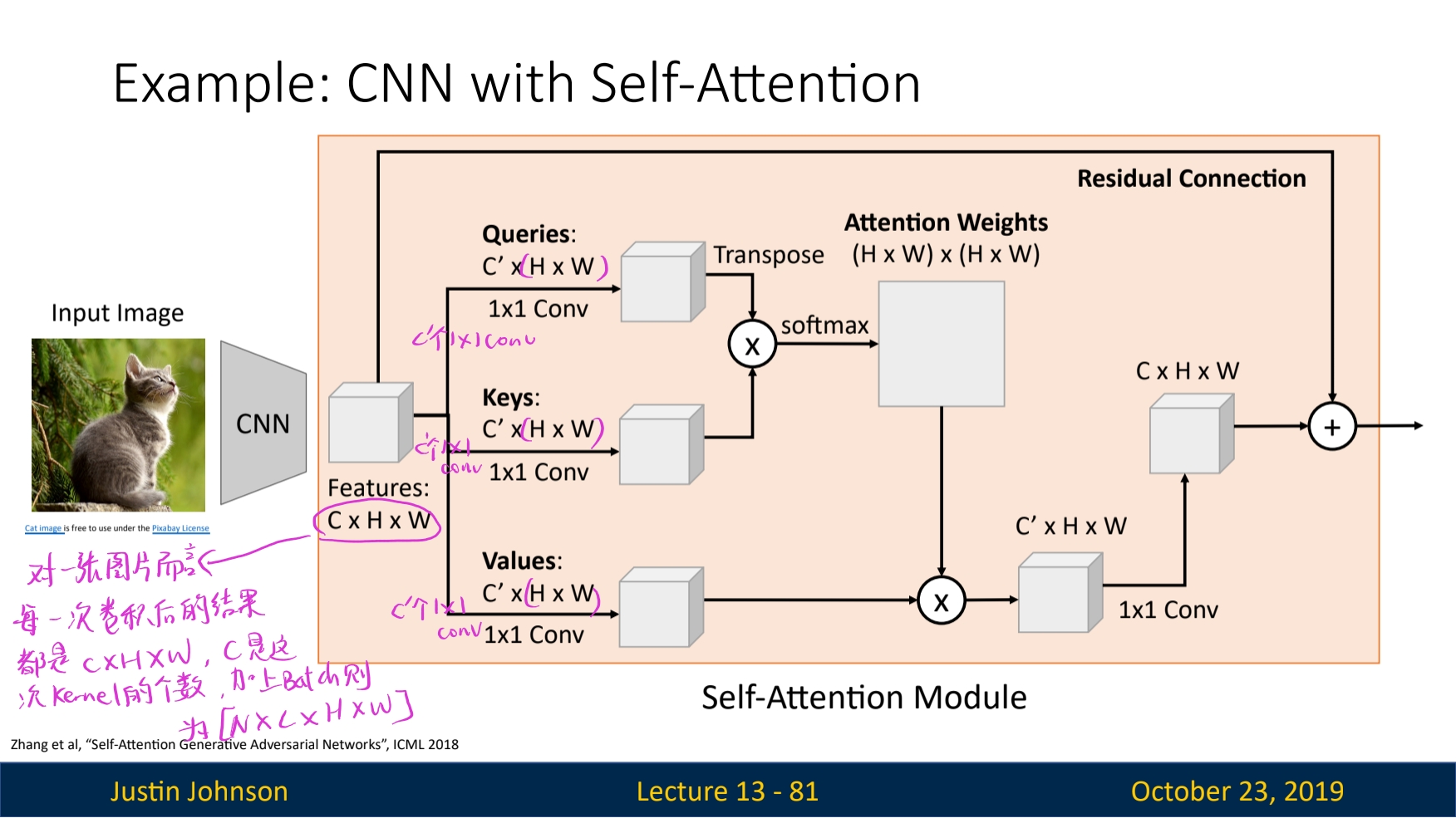
Conclusion on (Self-)Attention Model

The attention model solves the problem on tasks that input or output sequences. The essence of understanding sequences is that the generated output should take all the input (or corresponding hidden state) into consideration. We do can use vanilla RNNs . But they are hardly fit for large models. Self-Attention on the other hand fits for this request (a query vector compare to all input vectors), and is also more trainable.

The Transformer

We designed a new block that encapsulate Self-Attention model and use it do the sequence processing jobs. It is called the Transformer.

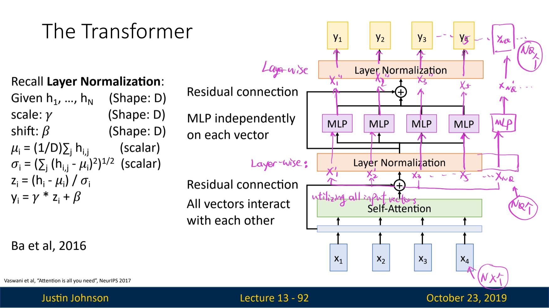
Hyperparameters: number of transformer blocks, output dimension of each block: $N_Q$ (also named in query depth, normally the same for each transformers) and heads(if we use the multi-head self-attention model)

The final structure is simply multiple cascaded transformers, as shown below:

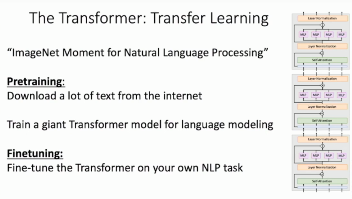
As the title of the paper inventing transformer, attention (by transformers) is all you need.