Generative Models
Generative Models
Introduction for Generative Models
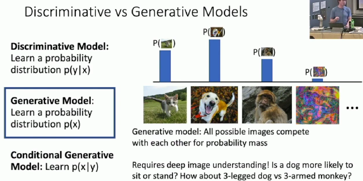
Definition
In definition, Generative models focus on image/pixel X, and tell the probability of X existing/occurring in the dataset. The mathematical principle is instead of training a model that tells a probability distribution of the labels, it tells the probability distribution of images, namely $P_X(x)$.
- It is different from conditional generative model(below), the model has learn the features of images themselves, without conditioning on captions / labels.
- And it is different from discriminative models(below), as the model output probability for images, not labels.
Applications
Generative Models are known for generating images rather than classifying them or captioning them. That is only a part of generative models’ applications.
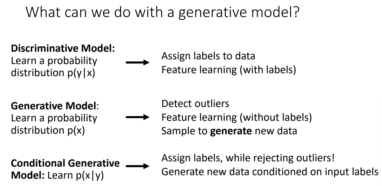
Above, x is the dataset of images, and y is the corresponding captions, descriptions or labels.
Detect outliers
When GM discover that one test point x has very low probability distribution over the dataset, it may not be the same category as all the images in the dataset.
Feature learning
Since in CV, our input can be images as well, therefore generative models are also capable of doing unsupervised learning tasks. And that foster GM’s abilities to learn very precise features and structures of input image dataset itself.
Sample to generate new data
We collect the model output, use techniques to reconstruct new images, and by definition they should resemble the images in the dataset.
Categories
The model has the same goal as to give a precise estimate of p(x). But the way of achieving this is different.
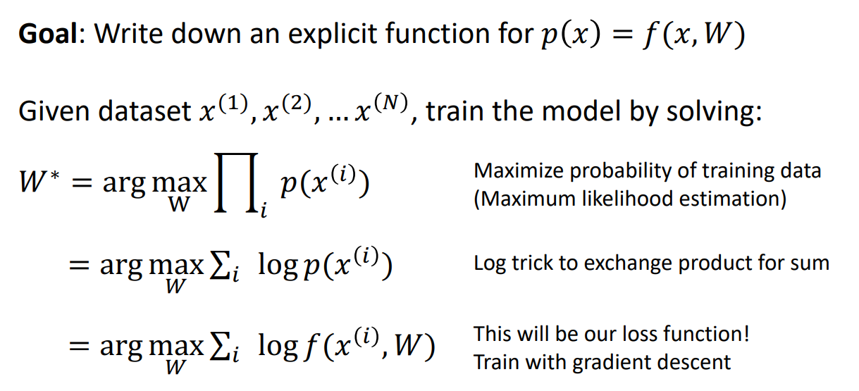
One way is by maximum likelihood estimation. And we design the MLE function with parameters $p(x) = f(x, W)$ so that we can maximize likelihood $p(x)$ by optimizing the MLE function, which is done by optimizing our parameters $W$ using data samples in our datasets (which is the neural network’s job). The creation of function $f$ is the essence of this explicit method. This correspond to categories of Column1s in below
Another way is still by maximum likelihood estimation to do the estimation. But when using MLE, we don’t design a $f$. Instead we design a lower bound $f_b$ for $p(x)$ which we hope similarly by optimizing $f_b$ , we can push up the maximum likelihood probability $p(x)$ and thus achieve good estimation. The idea of approximation is the essence of this method** This correspond to categories of Column2 in below
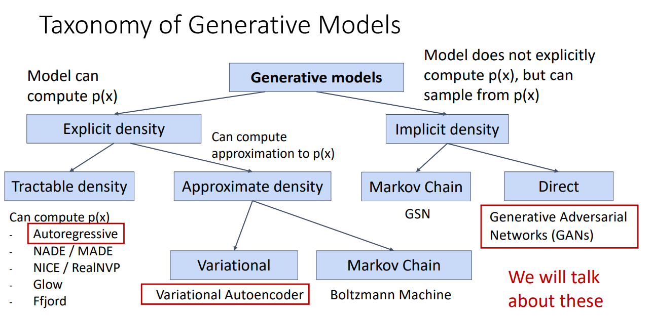
Examples of Generative Models
Autoregression Model
As its category shows, Autoregression Model figure out a way to design the maximum likelihood function, and therefore can use data samples to optimize the function (no labels needed in loss function!). The goal is given below.
So then how is the function designed?
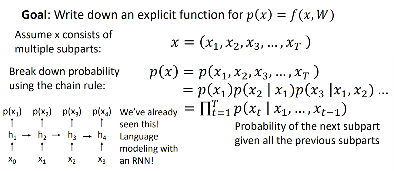
Autoregression model use probabilistic chain rules to rewrite the MLE probability. They also break images into pieces of pixels so that it fits in the chain rule function. Each $x_i$ corresponds to a pixel in $x$ (one big image sample squeezed to 1-dim). According to the formular, we multiply each probability of one pixel conditioning on the previous pixels, and then will compute the MLE function value.
The RNN structure perfectly fits for such network design. The combined architecture is called the PixelRNN as below
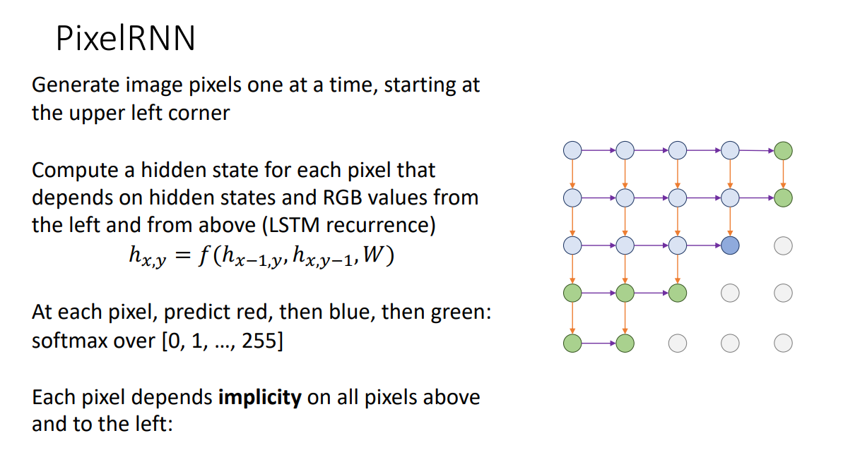
The problem is that it is as slow as RNN models.
Variational Autoencoders
As its category shows, Variational Autoencoders find out ways to compute the MLE’s lower bounds.
VA model does not come from scratch, it is from the idea of using autoencoders to build generative models. Autoencoders can already achieve learning features from image datasets along. But it has no way to generate probability distribution given its learned features. Previous researches only use these features for image captioning or other things.
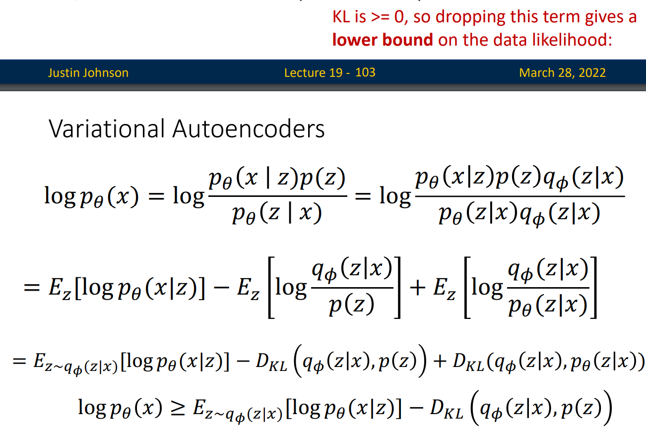
Variational Autoencoders help achieve image probability output. They design a method to compute logarithm maximum likelihood probability that fits autoencoders’ characteristics. Just unfortunately it can only achieve the lower bound of it. The formular and the symbolic meanings are given below:
Model Design
First level:
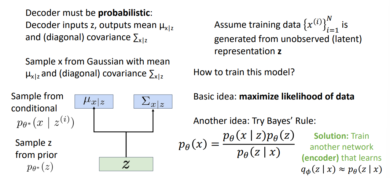
We want to utilize our features from the autoencoder and optimize our ability to estimate the MLE function, so we need to train a corresponding decoder for the job.
We choose the right basic formular and modify it.
- We relax the need for a probability output into assuming gaussian distribution and output the parameters for gaussian distribution.
- We replace the term with $p_{\theta} (z | x)$ in the Bayes’ rule because it is incomputable. It is the truth MLE value that autoencoder looks for. So we can only get a sample of such probability distribution from the autoencoder’s output, namely $q_{\theta}(z|x)$ .
- We assume the prior distribution of p(z) is trivial , of unit diagonal gaussian.
Second level:
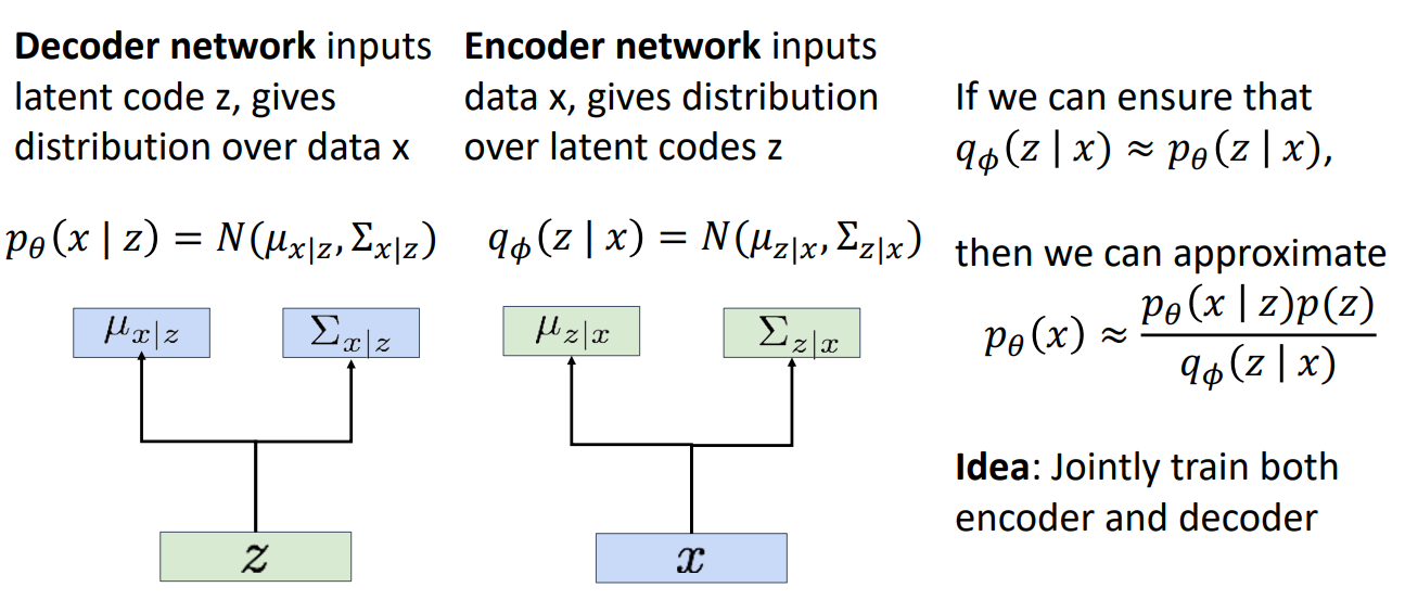
On discovering the fact that we need an encoder, we can move our design of the autoencoder here.
Third level:
We proceed to real mathematical induction.
The symbolic meanings for above ↓: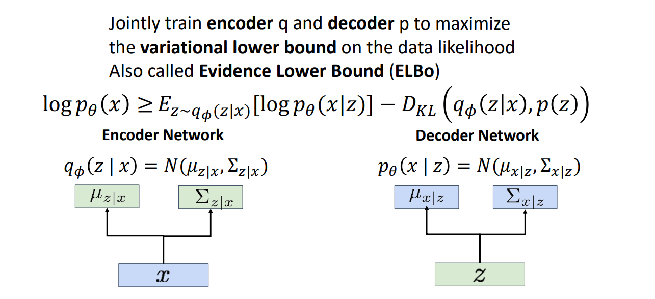
Why we use such formular? This formular is actually a bit complex, but it utilize a latent variable $z$ . We can express $z$ as a hidden feature inside image dataset, that fits for the job of an autoencoder.
Here is the intuition: So the lower bound is split into two terms needed for computation, the first respond to the efficiency of decoder model, which is how likely this latent variable $z$ can recover the original features, if z follows the distribution $q$ output from the autoencoder . The second term respond to efficiency of the autoencoder model, which is how far the output distribution of autoencoder differs from the actual distribution of $z$.
This result shows the design of our loss function and the architecture we will observe in training
Notice that we throw away the term with $p_{\theta} (z | x)$ in induction because it is incomputable, which is the same reason in level one.
Actually we don’t know $p(z)$ either, but based on real world facts, they are usually of trivial distributions like the unit (diagonal) gaussian.
Training
We use log MLE lower bound as loss function (see above), and train both decoder and encoder at the same time.

Testing
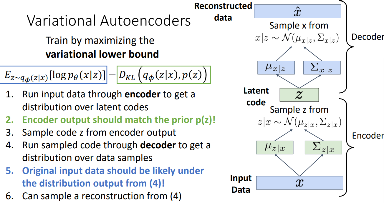
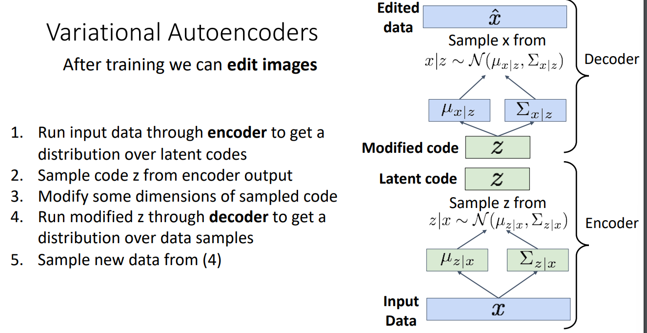
At test time, when we input one image, similarly we get an estimated distribution $q(x)$ from encoder, and we sample one $\hat z$ out of $q(x)$. We then use as input this latent variable $\hat z$ to the decoder. Finally we collect the probability output $\hat x$ which should be likely followed by the original input image $x$ . We sample from the output, and get the reconstructed image resembling the input image $x$.
Application
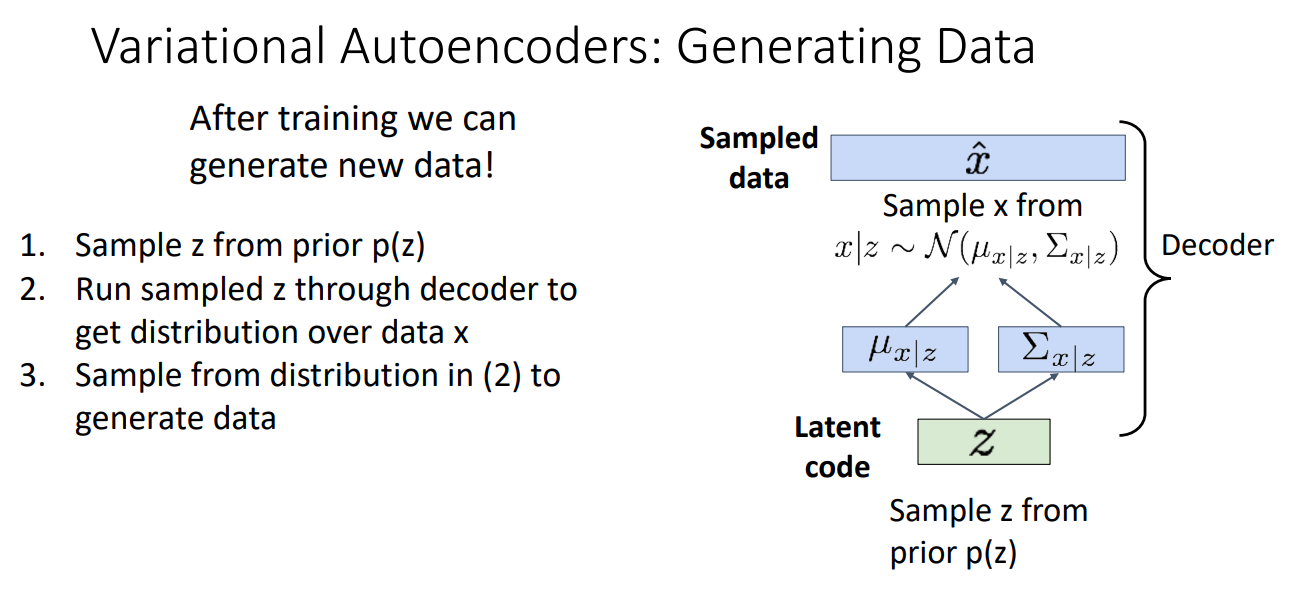
For image reconstruction, we throw away encoder, and just by sampling the prior p(z), we get a resembled picture output.
For image editing, we use encoder first to extract features. We can then modify them to edit the output images.
Generative Adversarial Networks
In VA model, the idea of adversarial networks actually exists. The encoder tries to compress the input data into more concise and simple information (more close to unit diagonal gaussian as we hypothesized), but the decoder want to recover the original image as much as possible (definitely harder if the input is less similar to the original image). The training goal of the two is contrary to each other, but training together kind of converge towards a universal optimal point for the goal of the output resembling input.
The term Adversarial exactly fit for the above condition, but GAN (generative adversarial networks) specific a more concrete class of problems.
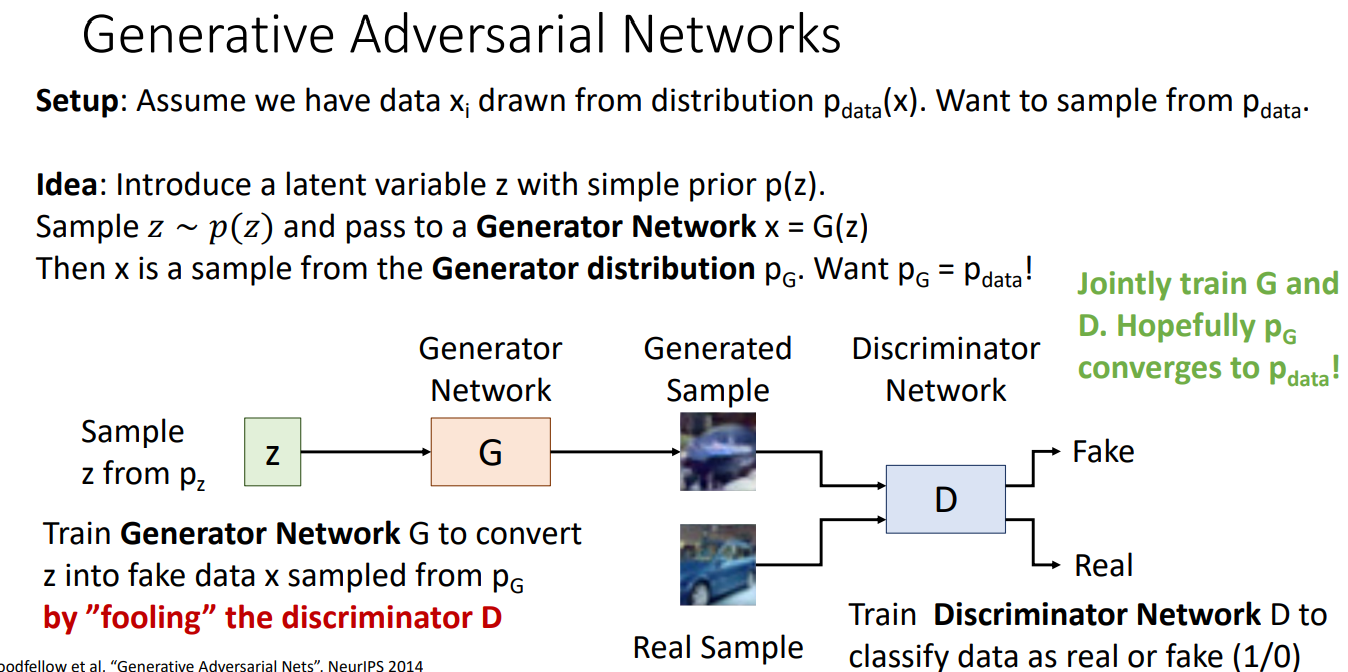
Classic GAN require the first model to be data generalizer that aims to generate as similar data as its input image in the dataset, while require the second model to be a binary classifier that aims to identify the input image to be whether generated or original image in the dataset as accurate as possible.
Adversarial exhibits in that the more similar the data is generated in the first model, the harder the second model will be to classifier then accurately.
The goal of GAN is to train the first model to output as similar image distribution as the input image distribution, or $p_{data} = p_G$
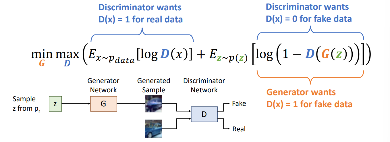
 We have a mathematical formular for the loss function for the classical GAN.
Optimality Analysis
For now we only get an intuitive idea that the two adversarial network tend to preform well. But whether minimizing the loss function will reach a optimum of $p_{data} = p_G$.
It turns out the minimum of loss function do guarantee $p_{data} = p_G$. Here is the proof.
We can first compute the inner maximum.
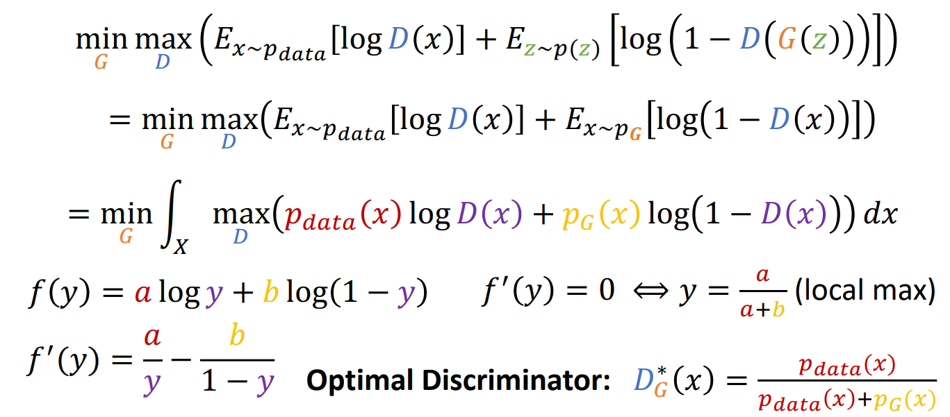
We find the inner maximum and plug in to get rid of maximum operation. Then we find something that we have researched already in Information Theory.
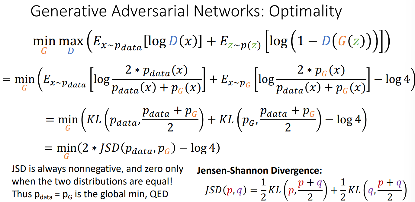
This is the overview of GAN, and for more detail please refer to the class video


