Reinforcement Learning

[toc]

Basic Setup

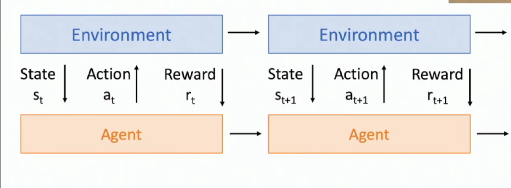
RL (Reinforcement Learning) consists of the following two components: an Agent and the Environment that the Agent is interacting with.

At each timestamp, the agent initiate to interact with the environment by sending an Action. The environment receive it and reply with a State and a Reward. The State contains the necessary information of the environment that the agent should use to make further Actions. The Reward can be any sort of things like a variable, a constant or another model. But all of them are designed to show how well the received Action is on considering reaching the final goal.

Such process unrolls through the time and form the basic structure of RL. So the natural goal of RL is to find the best action for the agent henceforth, given the received current state, and achieves the most reward from now on.

RL vs Supervised Learning

So concept in RL structure has an analogy to those in SL. Take the following illustration as an example.

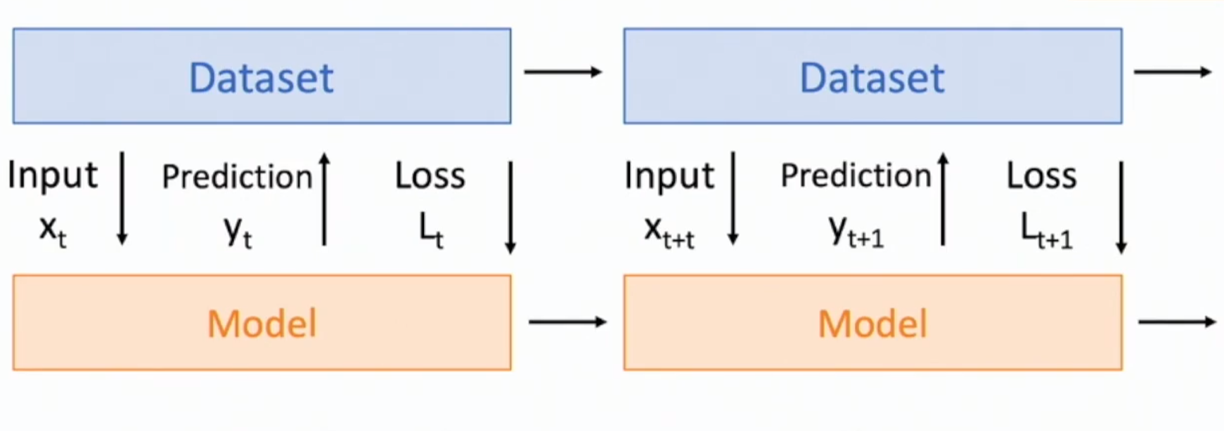
We can see the elements on the figure above can be paired with the one in the same location but in the above of above image.

There are several fundamental difference between RL and SL.

Stochasticity

We use deterministic functions to describe the process of SL whereas in RL we introduce probability. For example, we model the evolving step of the environment as a conditional probability.

Credit Assignment

In SL, we receive the feedback in one iteration instantly when the loss is calculated after the model makes a decision. But in RL, the reward in current timestamp may not entirely depend on the action made within this round. It may be a result of the comprehensive choices the agent has made over a long period of time.

Nondifferentiable

In RL, we cannot backprop through back the timeline and get the gradient of each action over its corresponded reward ($dr_t / da_t$), because we cannot have a certain function describing the stochastic change of e.g. the environment.

Nonstationary

The environment (the dataset in other word) varies as the agent learns. So the distribution of the dataset on which the agent is trained on is not stationary, which is the opposite in SL.

Introduce to RL Model

Markov Decision Process

Markov decision process evolves from Markov reward process which is induced from the basic Markov process.

A Blog describes such evolution very well: see here

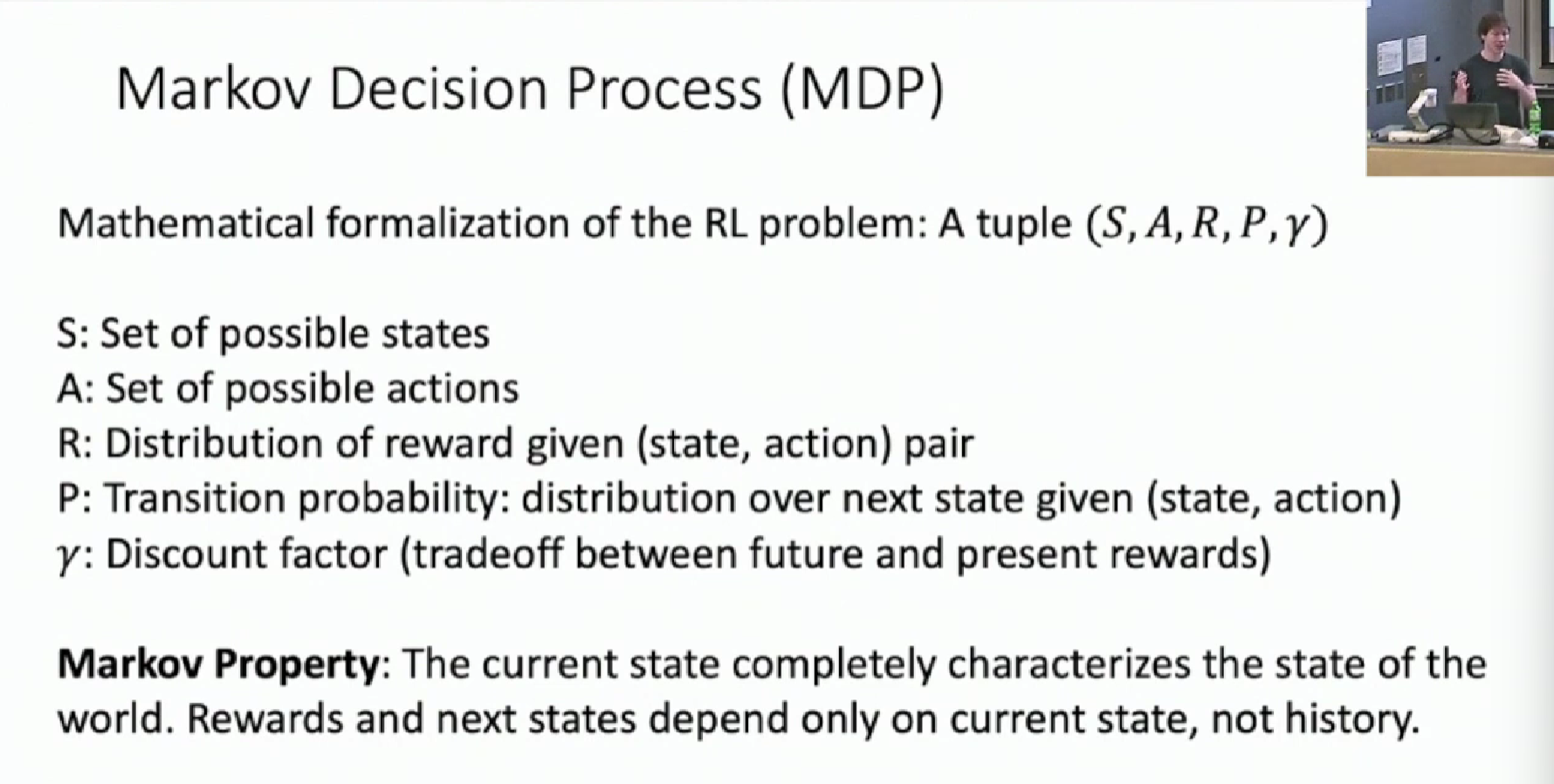
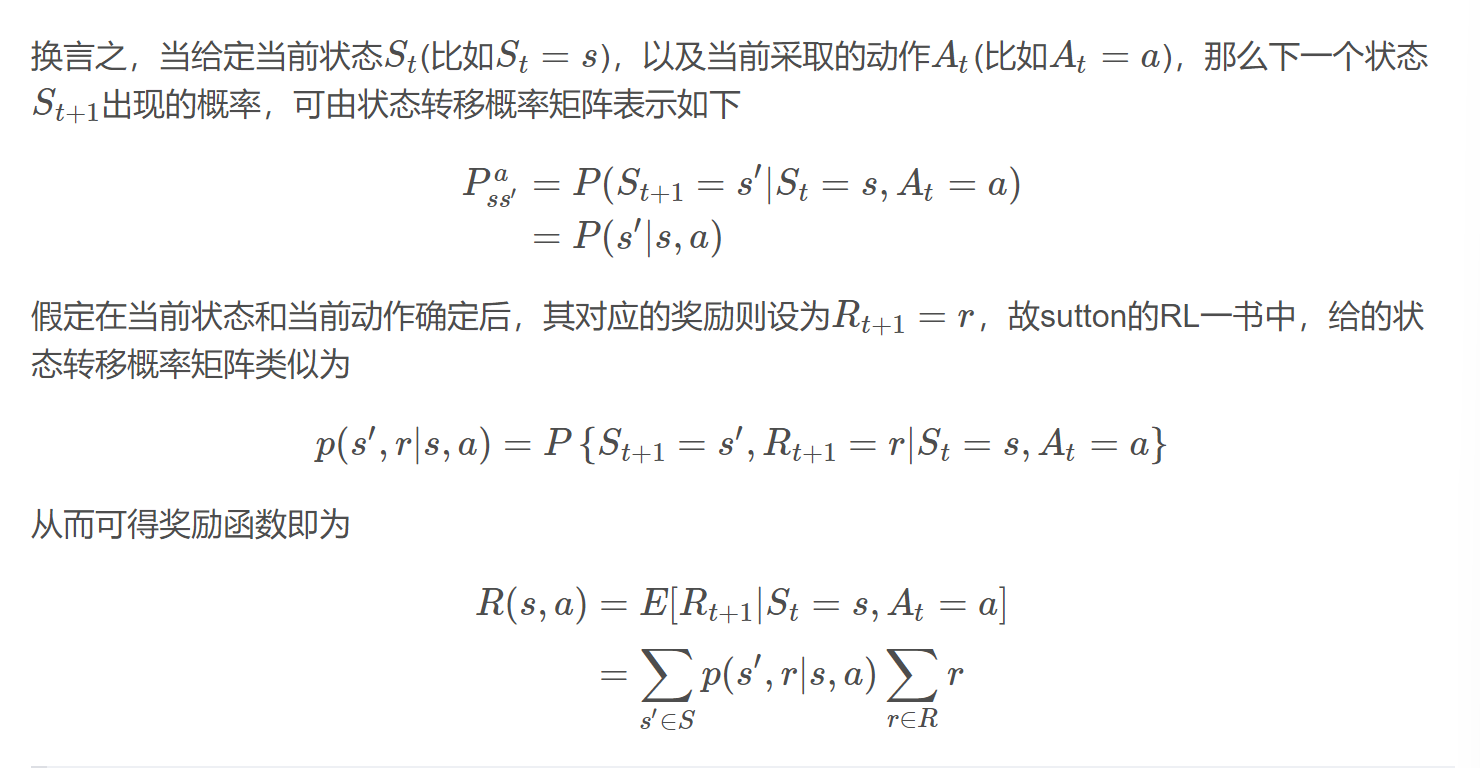
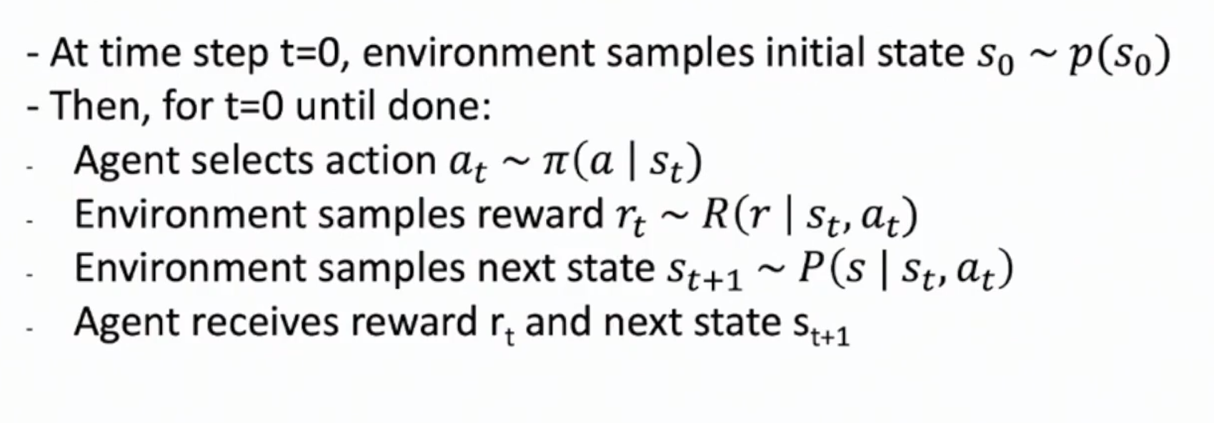
Simply put, the a Markov Chain uses a transition matrix at time t, $P_{t,ij} = P(u_{t+1, j} | u_{t,i})$ to describe the transition of the state at time t. For a MDP, the element in the state transition matrix at time t should be the probability of the next transitioned state $s_{t+1}$ conditioned on the current state $s_t$ and current received action $a_t$ from the agent. And in addition we can have a reward transition matrix which add the probability of giving reward $r_t$ into account.

Formalization of RL

MDP is used to formalize the Environment in RL.

And the agent’s behavior is characterized by a term called policy $\pi$, which is a distribution of actions conditioned on states

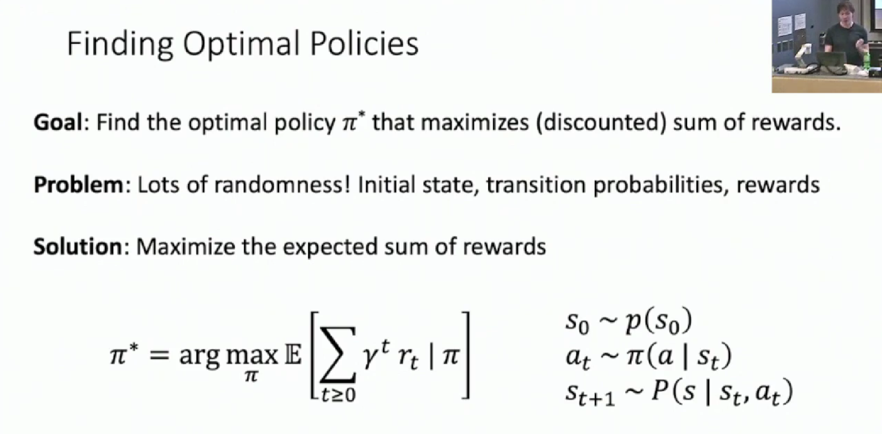
The Goal is the find an optimized policy $\pi^{ * }$ that maximize the cumulative discounted reward $\sum_t \gamma^t r_t$ (the reward we can get if following policy $\pi$ start from timestamp t)

Since RL deals with probability, the discounted reward is usually related to its expectation.

The idea is described below

Criteria in RL

Value Function

To analysis how good is a state, we propose the value function. It describe the cumulated rewards starting from state s , following policy distribution $\pi$.

Q Function

Q function tells us if we start from a state-action pair (rather than from a state only, as in the value function), and then follow the policy distribution $\pi$, what will the cumulated rewards be.

Bellman Equation

Given the goal that we need to learn the optimal policy function, we need a function to mathematically model the best policy distribution $\pi ^ * $ too. So we seek to the previous value function and Q function for help.

We define the Optimal Q-function as following:

$Q^{ * } (s_0,a_0)$ describes the reward of starting at $ (s_0,a_0)$ and then acting following the optimal policy $\pi^ * $. Thus we see the relationship between the $Q^{ * }$ function and $\pi^ * $, you just need to do the first action $a_0$ right! The following Equation describes it.
$$ {1}
\pi^*(s)=\arg \max _{a^{\prime}} Q^{*}\left(s, a^{\prime}\right) \label 1
$$
Then since we know that $Q^{ * }$ function already embodies $\pi ^ * $ function, then we can rewrite the definition of $Q^{ * } $ function as below, which is called the Bellman Equation

This shows the the optimal Q function has recurrence property. A recurrent version is given below.

But the most amazing property is the fact that: Any function Q we find that satisfies the Bellman Equation, must be the $Q^{ * }$ function And when we have got the optimal Q function, we can use it to perform the optimal policy it embodies.

**How to perform optimal policy given $Q^{ * }$ **

Based on the previous Eq.$\ref{1}{}$ , we can just perform the argmax over all possible action in current state. We find the best rewarded action and we can claim that is what the optimal policy $\pi^{ * } $ will take.

**How to understand the convergence of $Q$ to $Q^{ * }$ **

We are converging a function, and doing so by converge the value point by point, enumerating all the possible input space.

And the most brilliant thing is that, by starting at a random Q value for (s,a), iteratively doing the Bellman Equation, we will eventually converge to $Q^{ * } $ at this point (s,a)

Also the bad part is stated above. It is computationally impossible.

Training RL

Now that we have briefly introduced the basic concepts of RL, we proceed to how we train them. The core RL is to try to find the best rewarded policy $\pi ^ { * } $ . To do this, scientists have designed various algorithms, which form different types of RL variations. We will focus on two type of algorithm, Q-Learning which use Q function to indirectly depict the optimal policy distribution, and Policy Gradient, which directly models and solve the optimal policy distribution.

Q-Learning

In chapter [above](####Q function), we discussed the great potential of Q function to depict the optimal policy. We also mentioned that point-by-point converging the Q function is computationally unacceptable. We then give a neural network approach to solving the $Q^{ * } $ problem. We can call it the deep Q-Learning.

We can build a neural network with weight parameters to model the Q function. And we want to train it to fit the $Q^{ * }$ function. We can use the Bellman Equation to create our loss function. We hope after training, the model will function as the $Q^{ * } $ function, such as when we input the current state and action, the model output the numerical value which is the same as the $Q^{ * } $ function will spit out given the same input.

Let’s see how it is built in detail.

First, we set up our notations. we use $\theta$ to denote the trainable parameters in the formular. So we then need to train a network that approximate $Q^{ * }$ , or $Q^*(s, a) \approx Q(s, a ; \theta)$

Then we define how to train it, in other words, we should set up the loss function. We first show the outline.

Now we explain the above illustration.

First, we need to define the labeled data for each input state action pair. Our label data can be calculated from solving the Bellman Equation. Namely, for a given s and a and the model parameter $\theta$, we sample the next state $s’$ from the calculated distribution $P(s,a)$ and sample the reward $r$ from the calculated reward distribution $R(s,a)$ . ( See [MDP](###Markov Decision Process)). Then we do the expectation to get the output $y_{s,a,\theta}$ .

Then we get the output of our model, the $Q(s, a ; \theta)$. We then compare this Bellman Equation result with the result from model. Specifically, we use the square norm to compose the loss function.

Nonstationary Problem

In SL, although during training the loss value changes because the value of the model output will change, the label of an input data is fixed. Here however, the label of the same input data will also change through training, because it also contains trainable weight parameter $\theta$. This causes the nonstationary problem.

Policy Gradient

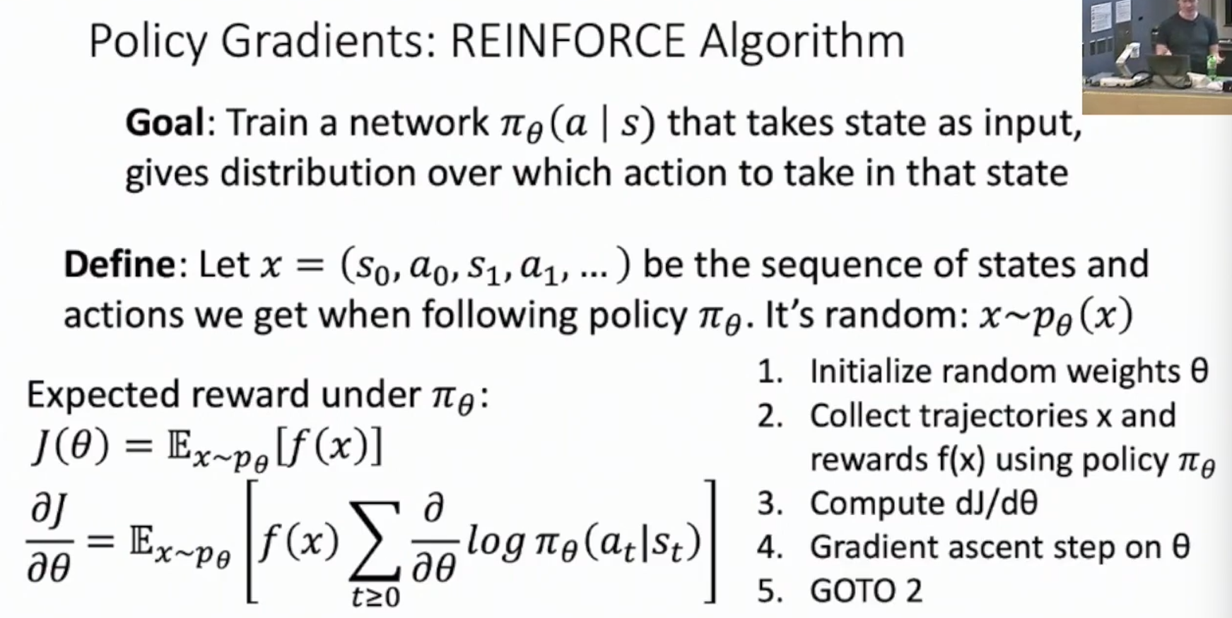
After all, the $Q^ { * } $ function is not the policy itself. We propose the idea of Policy Gradient model that **trains a network $\pi_{\theta} ( a | s ) $ that takes state as input, directly gives distribution over which action to take in that state.

The target function that we want to maximize is as following.

The idea is still the expected future rewards starting from time t, following policy $\pi _ {\theta}$ and collecting reward under the distribution $p_{\theta}$ calculated (conditioned on current state and action).

The problem is that we cannot directly compute $\frac{\partial J }{\partial \theta}$ because we don’t know the evolvement of the environment through time t, so it is a nondifferentiable equation.

To mathematically solve the problem, we perform the following things.

First we rewrite the formula. We first denote $x \sim p_{\theta}$ as the trajectory of our process, namely $x$ is a R.V. that is a sequence of R.V.s {s0, a0, s1, a1, s2, a2, …}, which follows the distribution $p_{\theta}$. And we define function $f$ , and $f(x)$ is the cumulated reward of the trajectory $x$. Then the general formula is

This $p_{\theta}$ is actually what we don’t want because it is related to the environment that haven’t been parametrized, and involves the trajectory over the whole process. Even we can describe mathematically use MDP (see after) so it is nondifferentiable, we can only sample it.

We want the gradient to do backprop, which is

In the final step, we assume that the reward function $f$ is independent to $\theta$. We managed to avoid taking the gradient of a nondifferentiable expectation, but we still cannot do such an integral over all the sample space of trajectory $x$. We need more simplification. The next step is as follow.

Now we reform the integral back to the expectation, which is operable via sampling!

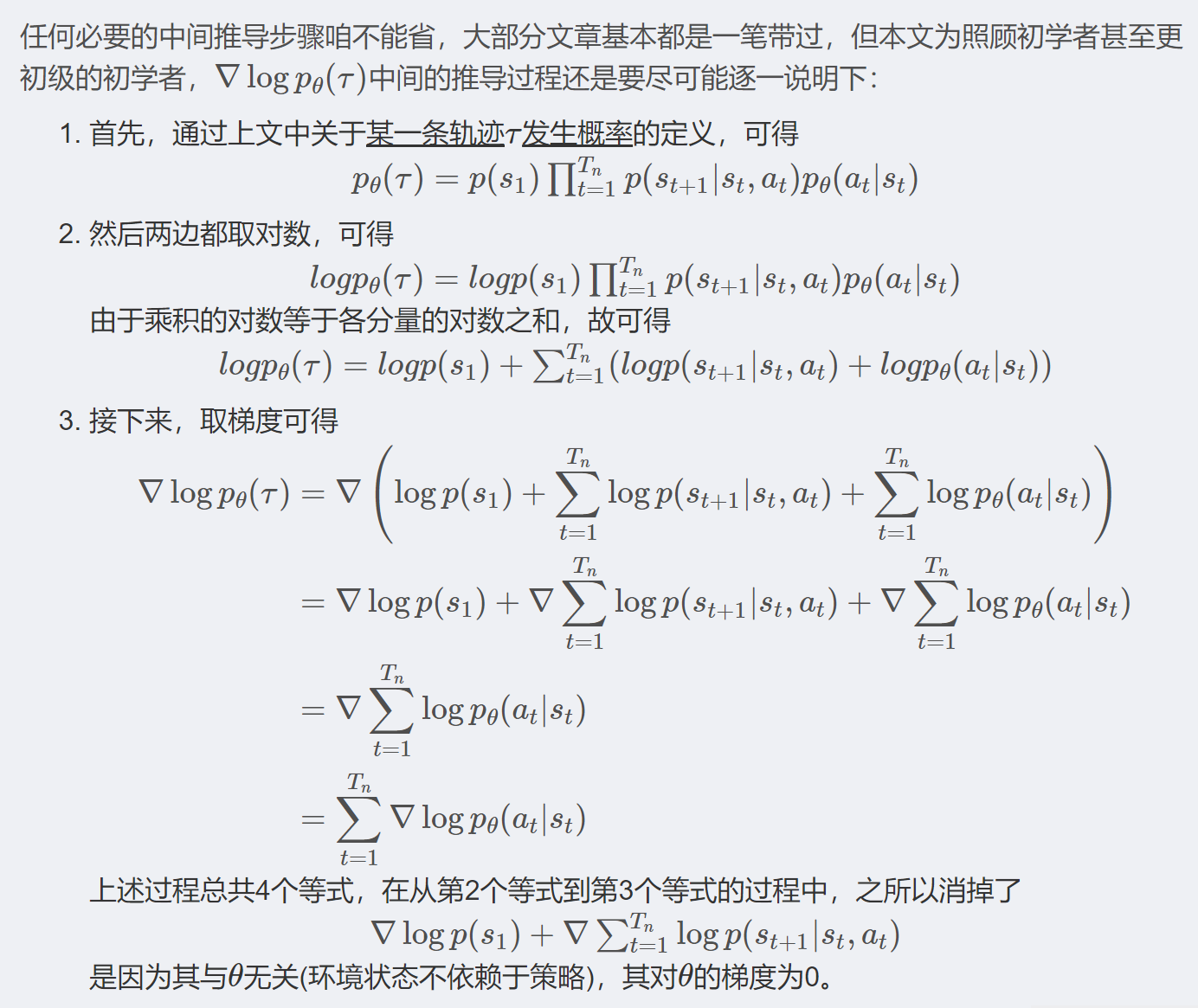
Finally we have to think of solving the term $\frac{\partial}{\partial \theta} \log p_\theta(x)$ inside the expectation. The steps are as follow.

Errata: $p(s_{t+1} | s_t)$ should be $p(s_{t+1} | s_t, a_t)$ . But the result remain unchanged. **The change of Policy does not influence The change of transition of environment state. **. The gradient is still zero.

In the illustration above, we start from the definition of $p_{\theta}(x)$. By the MDP property we unroll the formula of $p_{\theta}(x)$. We do the logarithm and compute the partial derivatives. Then we find the term with respect to the change of environment can be discarded in the partial derivatives because The change of Policy does not influence The change of transition of environment state.

A detailed deduction is given below

In all, we get our final formula on how to compute the gradient of target function $J$ (the cumulated reward function).

To compute this, we just sample the trajectory $x$, following current policy $\pi_{\theta}$ and collect the rewards to compute $f$. With respect to the gradient of the predicted action score $\frac{\partial}{\partial \theta} \log \pi_\theta\left(a_t \mid s_t\right)$, since our model’s job is to output the policy (the distribution of next action over current state), we just need to backprop back through the model to compute the gradients.

Therefore, the overall training scheme can be as follow.

Other Approaches

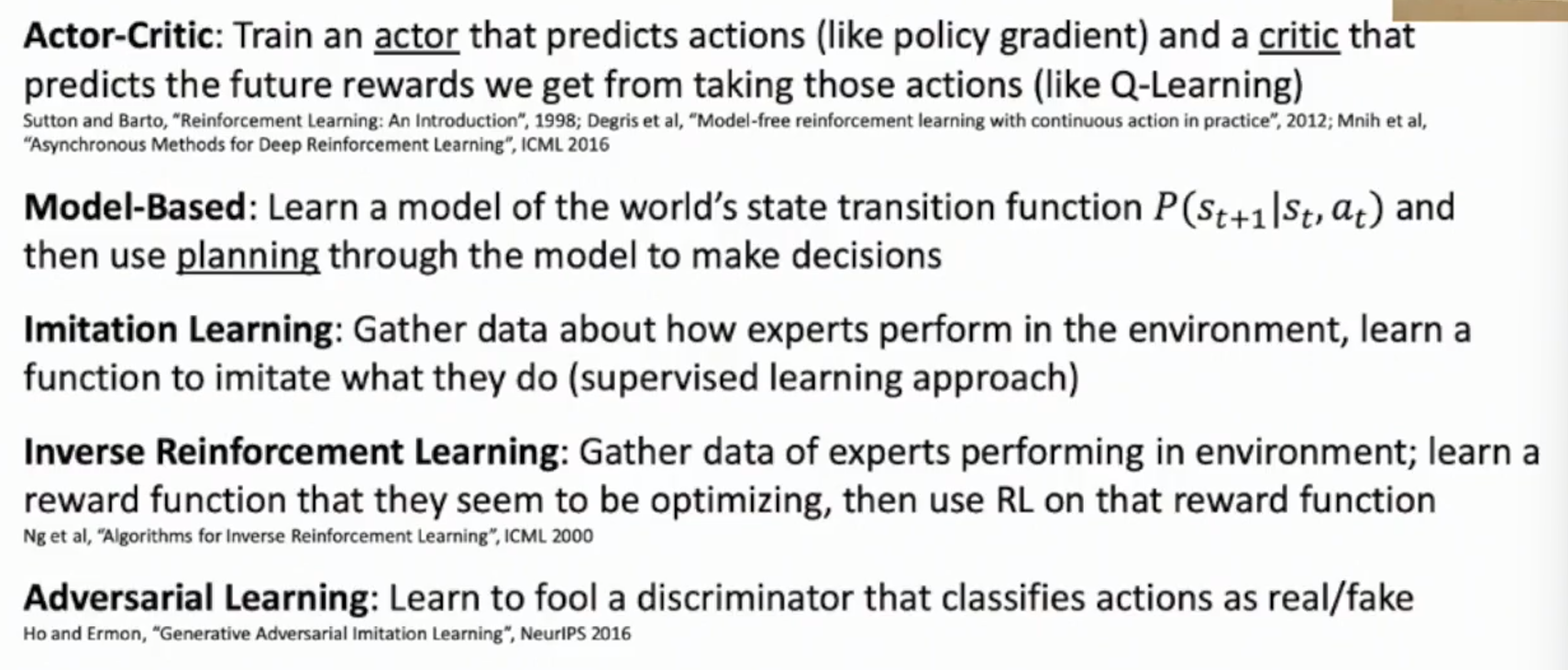
As said before, there are a lot of choice on the variations of RL.

• Actor-Critic: The main model for finding policies is still Policy Gradient, but the reward is predicted by a trained Q-Learning model (use Q function to evaluate the current (s,a) pair is good or not, where s is the current state, and a is the action predicted by the Policy Gradient model)
• Model-Based: We can train a model to depict the environment, specifically, the transition of the environment, and then use planning through the model to make decisions.
• Imitation Learning: We can gather data on how human choose their action and just train the model like a supervised learning, whose label is the sequence of human operations.
• Inverse Reinforcement Learning: We can use human interaction data to train a RM model that give rewards (like in RLHF, the RM model is trained using supervised learning to learn to arrange the exact rank of answers from ChatGPT. The output is that, the more similar to human arranged orders, the higher the reward is) Then we train the RL using other methods but using the trained RM model.
• Adversarial Learning: see above.