Diffusion Model (I)

Introduction

The sculpture is already complete within the marble block, before I start my work. It is already there, I just have to chisel away the superfluous material. – Michelangelo

We can shortly describe the diffusion model as a text-to-image generative model using a denoise process which utilizes diffusion.

From the concept above, we simplify two concept that is crucial but typical to the diffusion model, the Denoise Model and the Text-to-Image Layer. We will discuss them in the first section.

But to achieve a matured generative model, we need a more complicated design. Therefore, explanation for other part of the network and how they are modified and assembled together as a well-functioning model will be elaborated in the next section. The mathematical principle will be discussed in the third section.

Let’s proceed to introduce the first concept, the denoise model.

Denoise Model

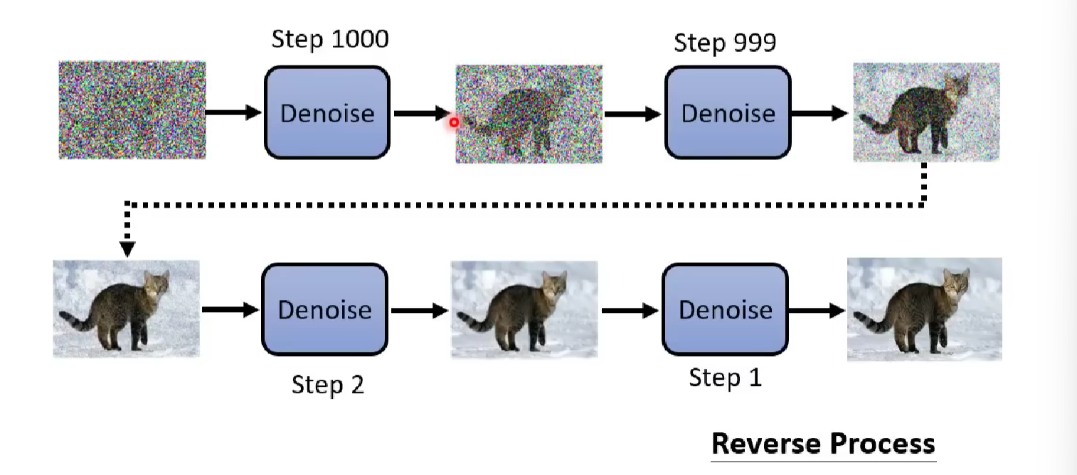
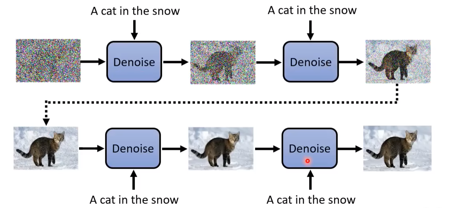
A simple wrap up for the denoise model is that, first we sample a tensor with the same dimension as that of your desired photo from the normal distribution. Then run the denoise model for a fixed number of steps. After steps of processing, the photo looks more close to the photo that you described or desired.

We first look at how the model is designed, then we proceed to how to train it and the its principles.

Model Design

As said before, the denoise model is the core to generating photos. Actually we only have one denoise model in one diffusion process. During application, We just iteratively send the previous output as the input of the denoise model in the current round to generally denoise towards a clear picture.

To make sure the denoise model is aware of the current process, the input of the denoise model is the previous output photo and an additional timestamp which mark the current denoise step.

That is not the whole story, for a text-to-image application, an additional text prompt may add to the input of the denoise model. We will talk about it later

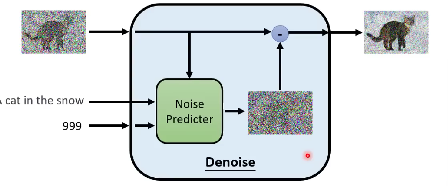
Here is an inside structure of the denoise model

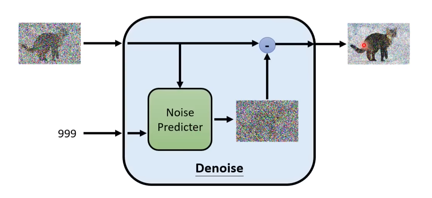
A denoise model at timestamp t generate a predicted noise image given its input. Then we subtract the predicted noise from the input previous photo, and get our output, which is a relatively clearer photo. We call it the denoise process.

But we not yet understand how it is trained.

Detailed Implementation

To analysis the implementation of denoise model, we should always look at two ways of the model.

• The forward process (diffusion process) provide the ground truth to train a noise predicter used in the denoise process.
• The backward process (denoise process) generate the image from Gaussian noise input during application, using the noise predicter and subtraction, aka the whole denoise model.
• The denoise model is the combination of the noise predicter and subtraction gate.

Three basic component of the denoise model ↑

The denoise process is mentioned in the previous sector. Now, let’s look at the diffusion process.

To train the noise predicter whose output is actually the predicted noise photo, we have to think about how to collect its ground truth.

The illustration shows how we use a diffusion process on a clear photo, and then use it to train our noise predicter.

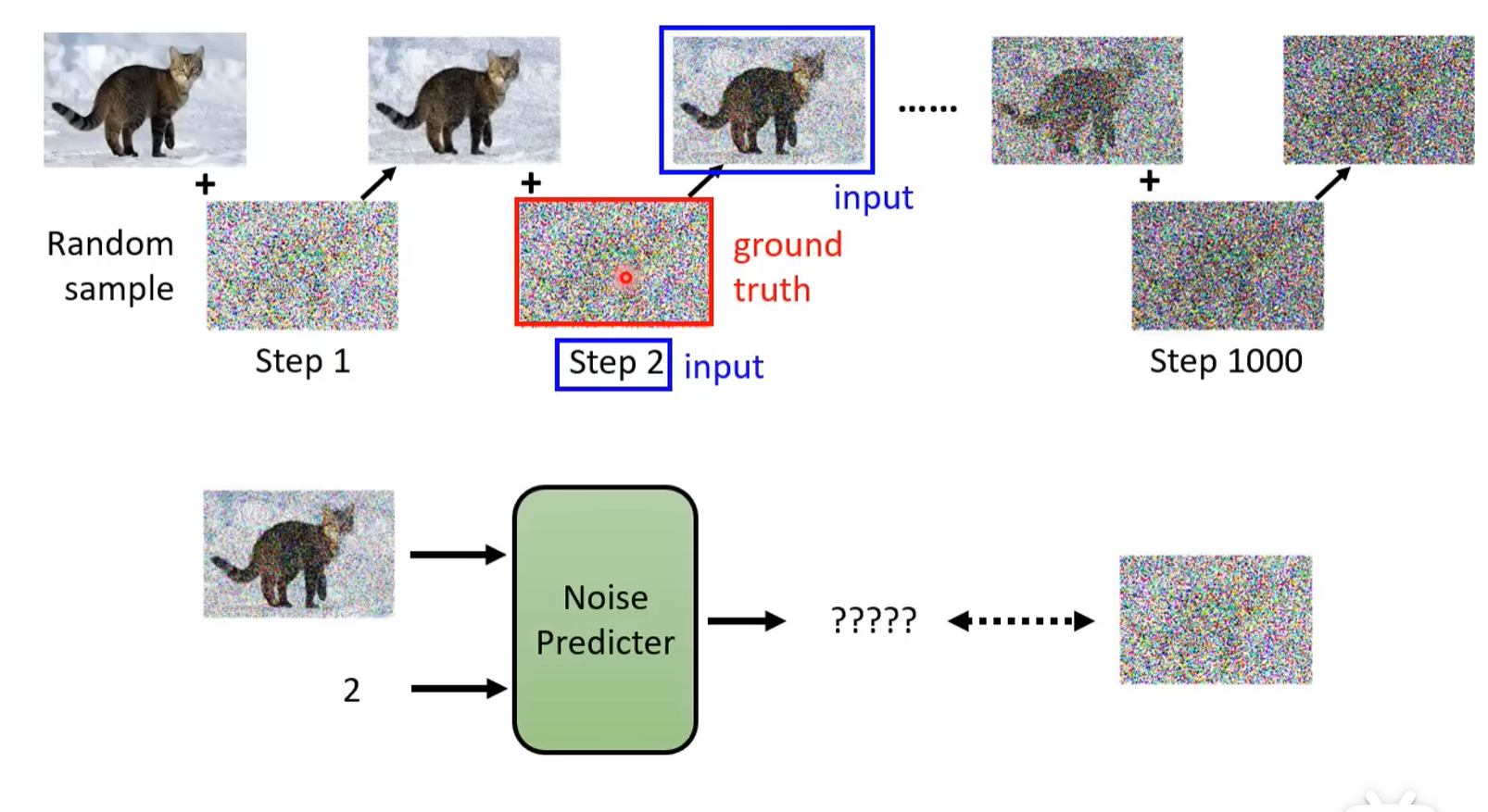
The diffusion process is done by random sampling the previous diffused output and get the noisy image, then add it to get the current diffused output.

To train the noise predicter, the blue square is then the input to the noise predicter, while the ground truth is the required labeled data. Specifically, we use timestamp and diffused output as input, and the noise image at each timestamp as the ground truth.

Text-to-Image Layer

For the first step, we need to let the model understand the relationship between text and picture. We need many paired data, and then can we add another input dimension, the labeled text, to the denoiser and use the paired image as the ground truth data of the first image in the diffusion process.

Specifically, we want the denoiser to be trained to generate the noisy photo with respect to our prompt input, previous denoised photo, and timestamp.

The noise predicter in the denoiser should be changed simultaneously

The Framework

In real diffusion model architecture, we use a encoder-decoder like structure to do the text-to-image generation.

We first introduce the new architecture, then we compare it with that in the first section.

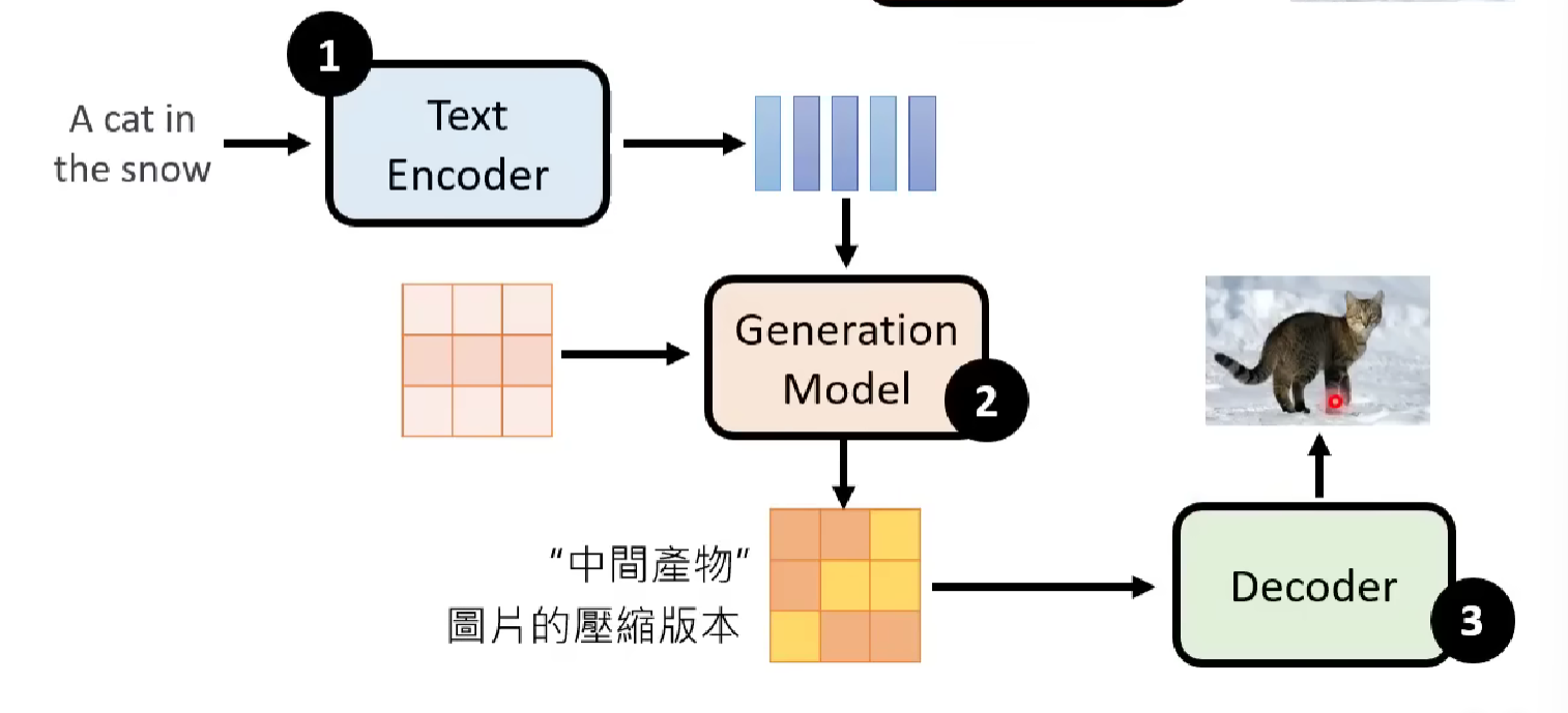
The first component is the text encoder, which translate the natural language into machine-used word-embedding vector space.

Then a generation model such as the diffusion model is used to generate a latent variable vector (containing the compressed information of the target photo, could be a small size version of the target photo, or things only the decoder understand, completely depend on the design of particular model) from the input, the first sampled noise vector and the processed prompt from word vector space. In this step, the information is transferred from the word vector space to a latent variable (or we say a compressed photo) in the latent space, which we believe to have concentrated the information over the entire image space.

In the last step, we use a decoder that can interpret the latent variable into the target photo.

This latent space is the same meaning as that in the VAE model, which is all a part of the latent variable model category.

But unlike the VAE model or the Transformer etc. , for text-to-image application, we tend to train the three component separately.

Here are several famous model architecture using the encoder-decoder layout.

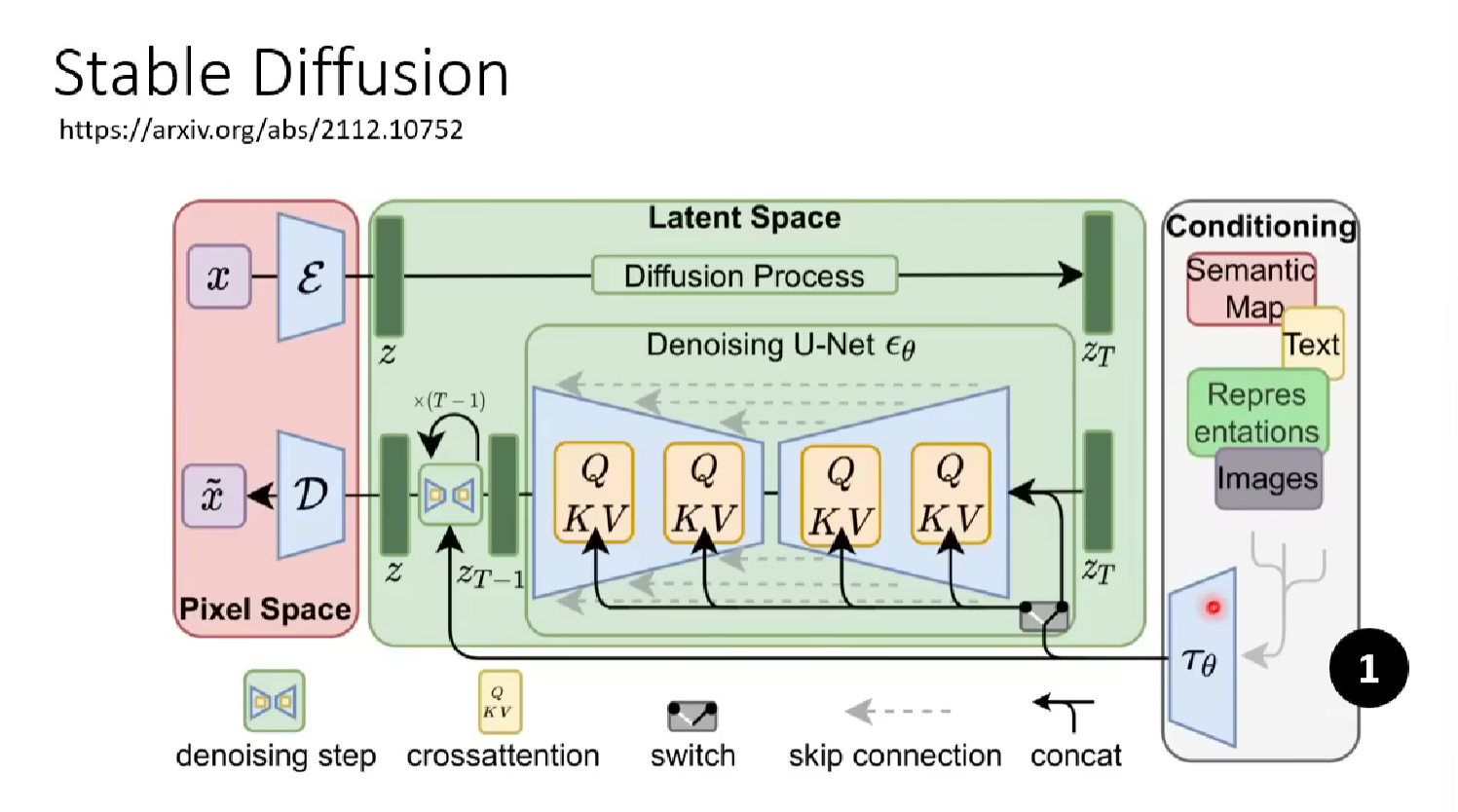
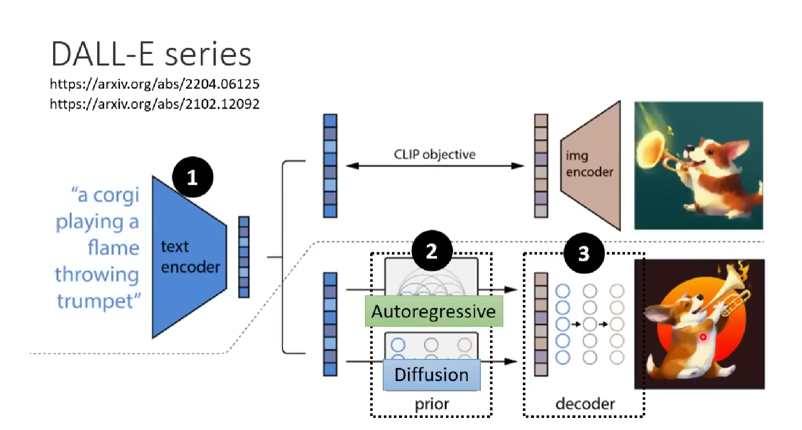
Note that the autoregressive model is experimented in DALL model. It perform decently, because we use a decoder so we don’t require the generative model to do the whole model generation job.

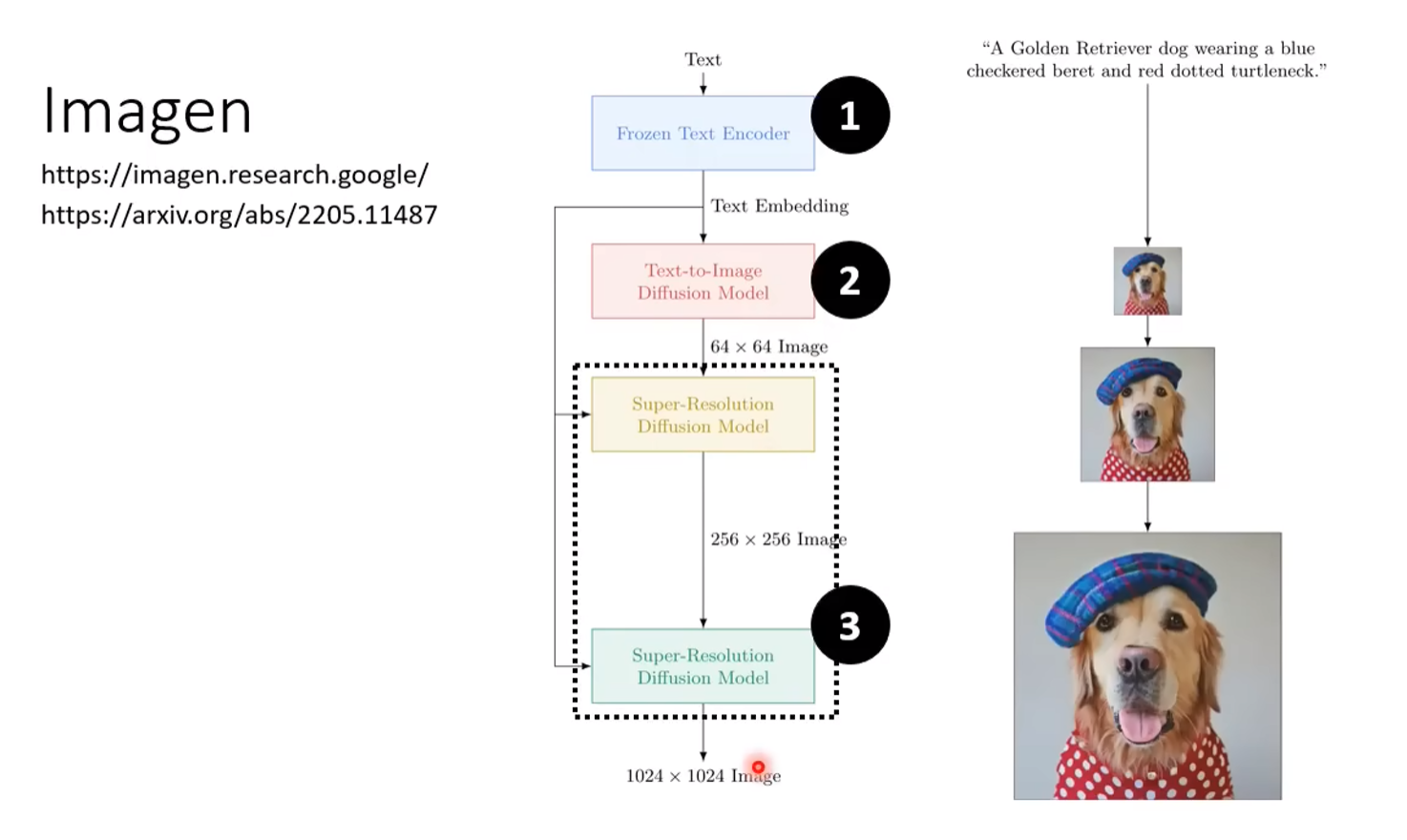
Text-Encoder

According to the lecture, you can use almost any LLM training process to serve as your text-encoder. The function is correspond to the text-to-image layer in section one.

Recall that in the article about BERT, we conclude that the pretraining of these LLMs is actually training the weight parameters in the model, or the word embedding and weight matrixs in the model.

In the article about GPT, we even see how OpenAI arranged the input data scheme for various downstream tasks, without modifying the pretrained model.

Thus I think it is reasonable that the lecturer says we can use LLMs to be the text-encoder, which we only need the embedded word vector space for downstream generation tasks.

In the article of Imagen, Google conducted an experiment saying that the choice of Text-Encoder is crucial to the final result of the generation model.

Since Google’s paper emphasized on the importance of Text-Encoder, we can discuss a bit on the criteria of distinguish a good and a bad generative model.

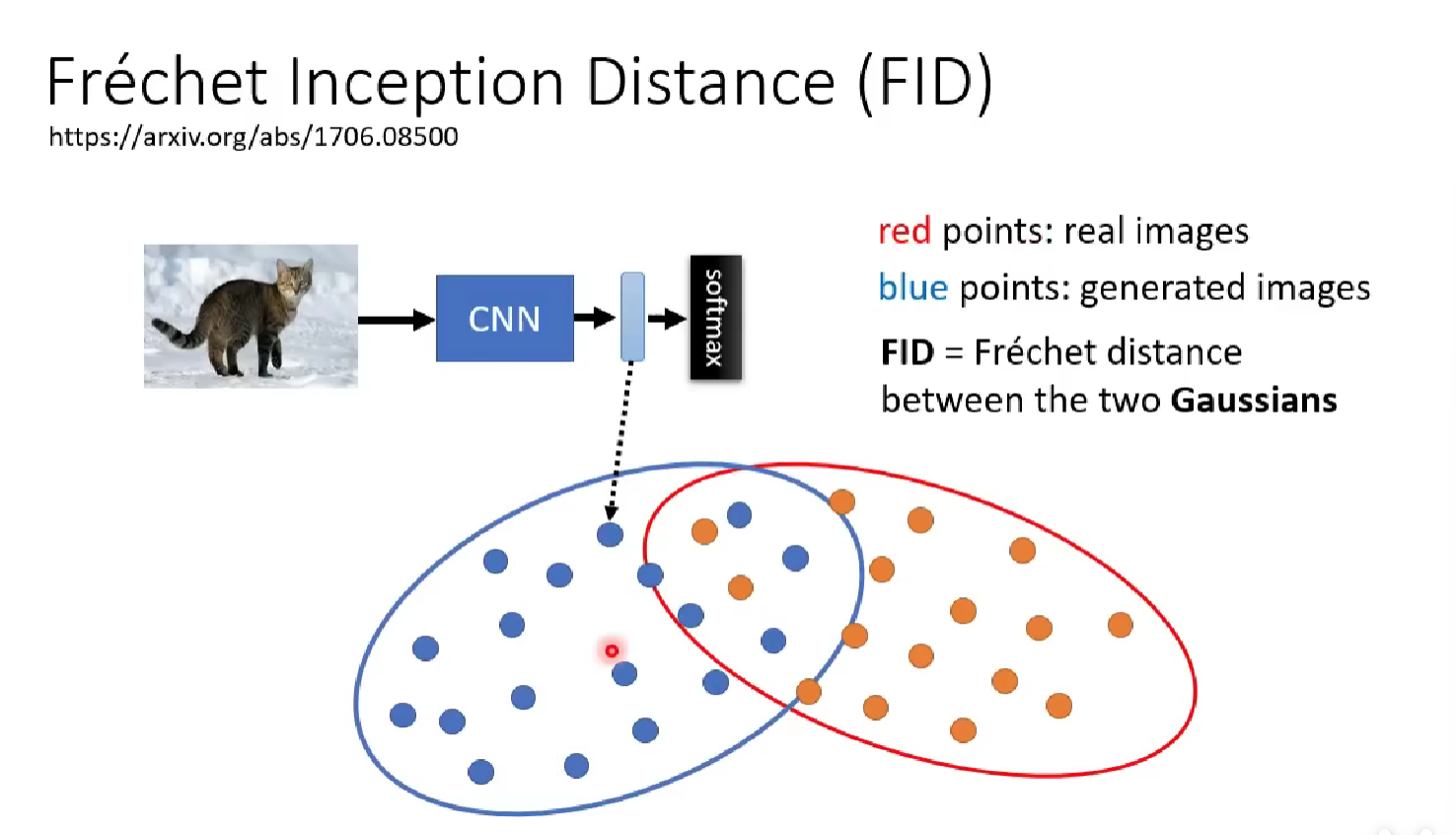
Fréchet Inception Distance (FID)

FID compares the Fréchet distance between the two distributions, the latent space (feature space) of the image generated by the model and that for the genuine images. The larger the distance, the less likely the generated image resembles the real one, the less the capability of the model is.

But how to get the feature space of the two kind of image? (If we have experience of GAN or Face recognition, the use of such technique may be familiar to us)

We can train a CNN model that input with all our data, and get rid of the final classification layer (one FC + one SoftMax). The model then is known as a feature extractor which output the representation of the input image in the feature space of all the input data. Then we input again some generated images and genuine images to sample out the two distributions from the feature space. After we input enough photo and sample enough from the two representation, we perform the next step, comparing the Fréchet distance.

To make comparison, we must assume that the two distribution are actually Gaussians. This is nontrivial but the fact is it works well on many examples ( close to human results). So we let it happen. Then we can perform Fréchet comparison according to some algorithm, which is omitted here.

Contrastive Language-Image Pre-Training (CLIP)

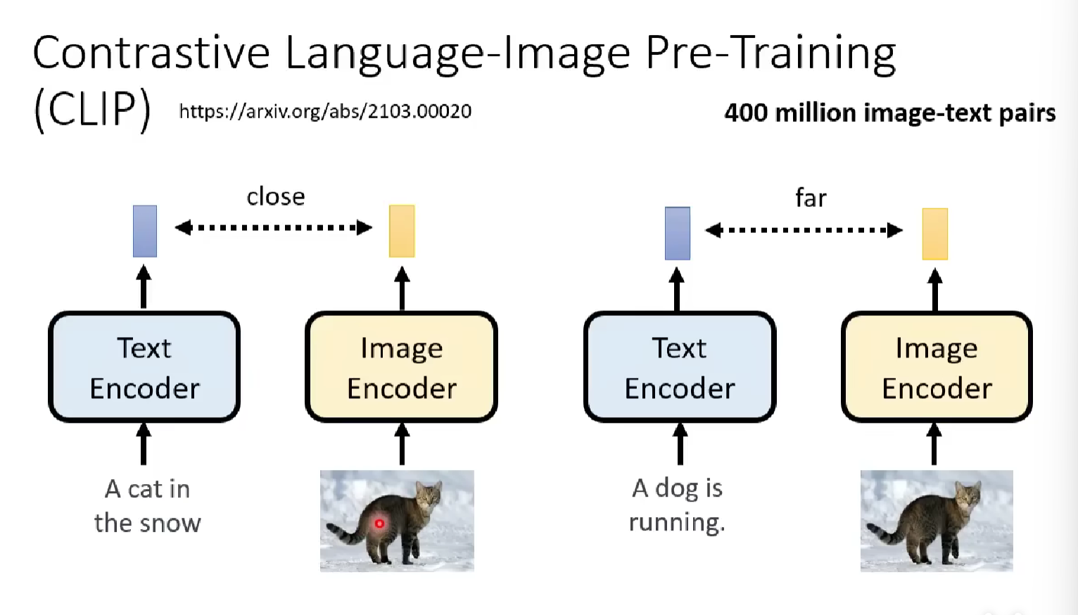
CLIP is a model pretrained to compare the relativity between the text and the generated image.

It has a text encoder that can receive the input natural language text and output the encoded text vector.

It also has an image encoder that can receive a image and output the encoded image vector.

If the text vector and the image vector has a close distance in between, that means they are relevant ( or naturally they describe the same thing), the score given by CLIP will be high, otherwise the score will be low.

Therefore we can use CLIP to supervise whether our model produce images that is close to the text prompt input. You just input the generated image to the image encoder and the text to the decoder, then let CLIP judge it for you.

Decoder

Recall previously we say that the decoder generates the image based on the latent representation of the target image, provided by the output of the generative model. Then based on different type of decoder, we can will design different training scheme and target. But there are a common ground among all of them: they can all train without labeled data (no text-image data pairs, just images), more specifically, self-supervised learning. Here are some examples.

If your decoder input a compressed image and output the finer and larger version image, you can create the input by down-sampling the original image, and train the model to generate the output as much alike as the original one.

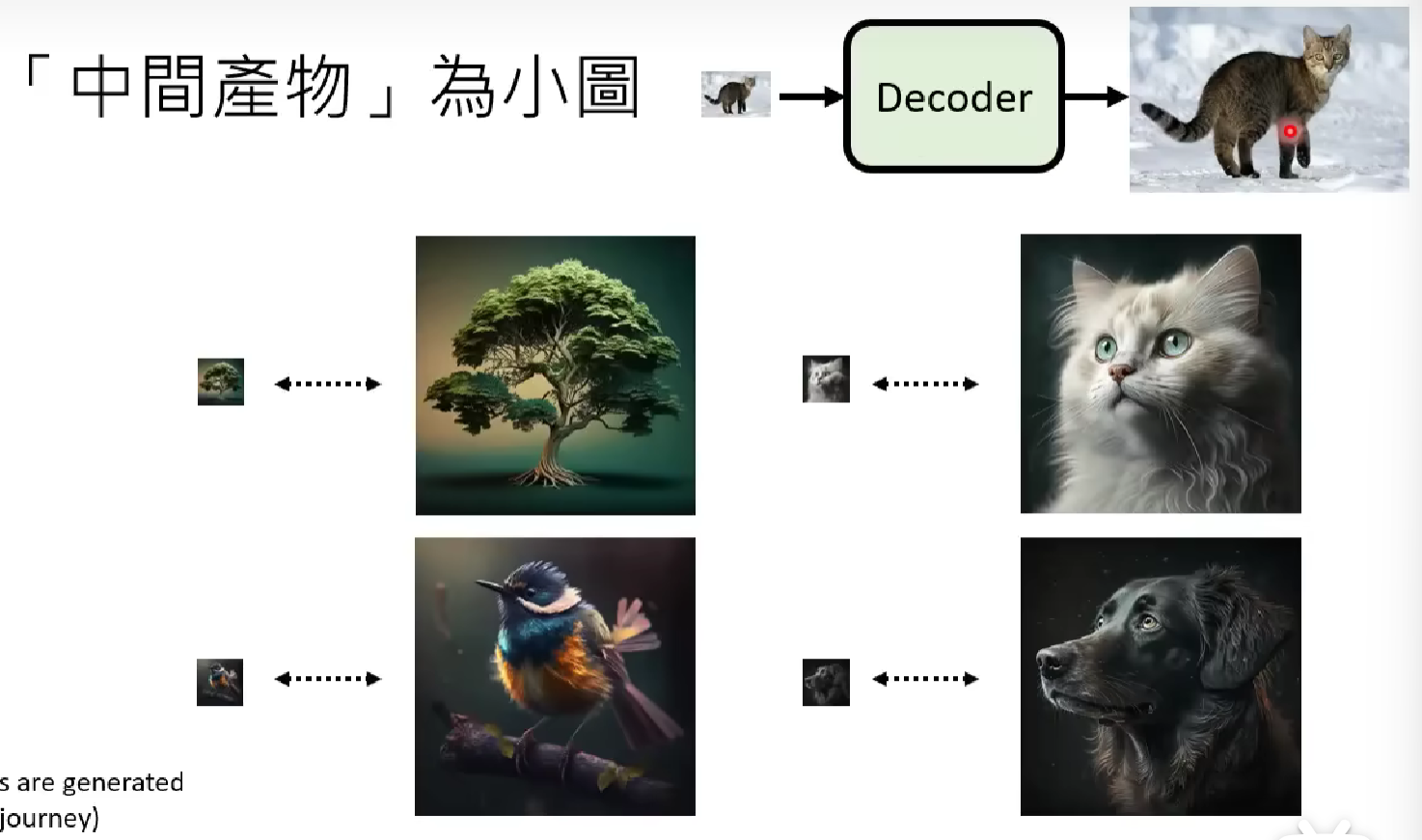
If your decoder input a latent representation, you can use the auto-encoder model to train that decoder for you. The setup of the auto encoder is mentioned in the article about VAE. The difference between VAE and AE is mostly that VAE output the probability of the target image, where as AE’s decoder is truly responsible for generating a picture.

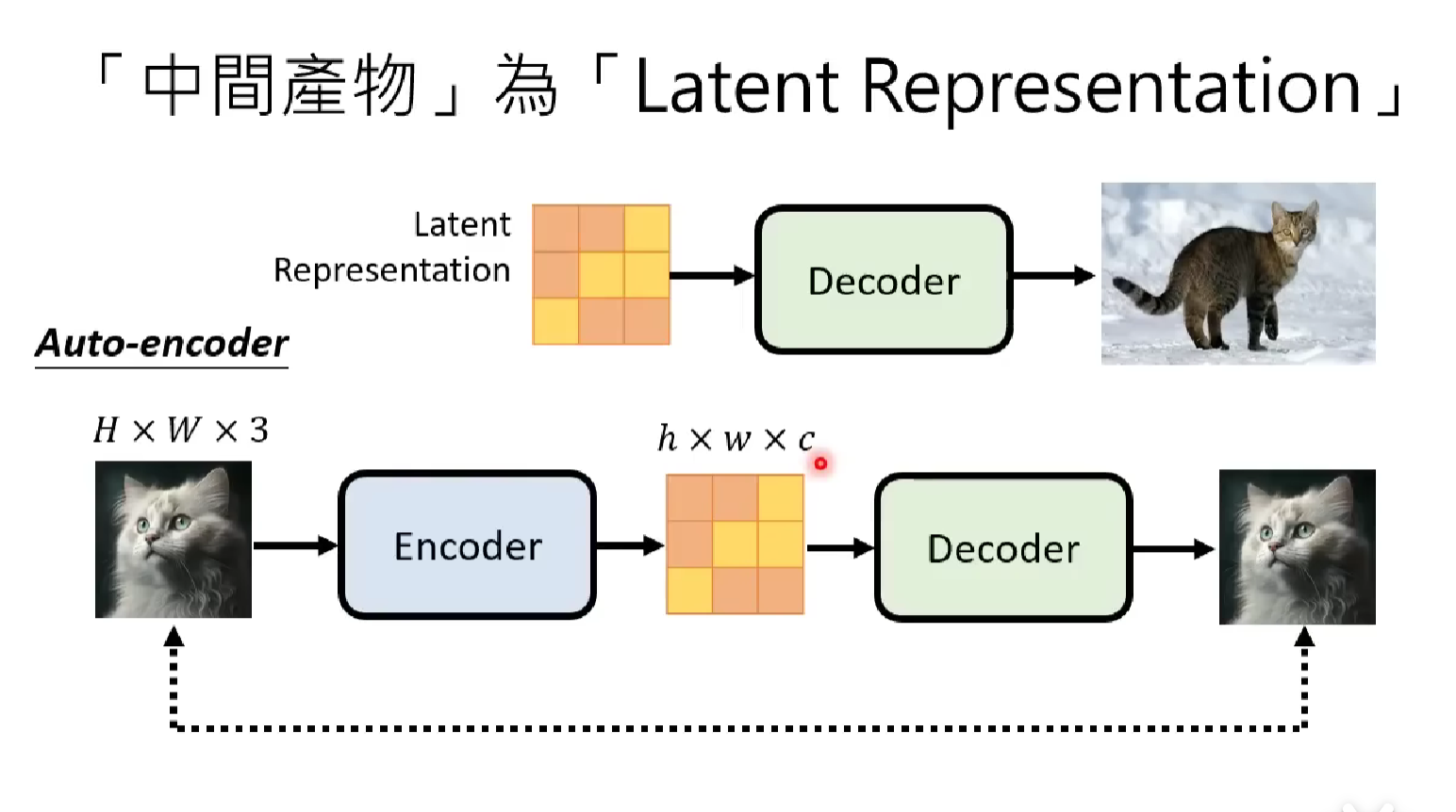
The latter is adopted by more modern model architecture like Stable Diffusion and DALL-E.

Generation Model (Denoise Model)

The generation model as a whole input the encoded text representation and a noise. We use the diffusion based denoised model in this section. Many of the concept is the same as the Denoise Model section above.

To analysis the implementation of denoise model, we should always look at three part of the model (two-way process + one model design).

• The forward process (diffusion process) provides the ground truth and trains a noise predicter used in the denoise process.
• The backward process (denoise process) generates the image from Gaussian noise input during application, using the noise predicter and subtraction, aka the whole denoise model.
• The denoise model is the combination of the noise predicter and subtraction gate.

The following illustration provides the overall structure of the pretraining of the diffusion model, equal to the diffusion process above.

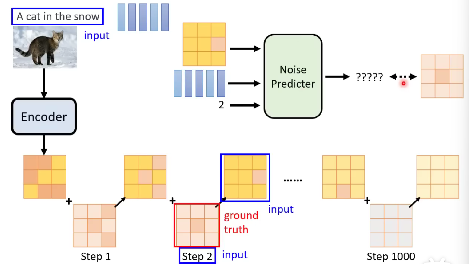
Let’s break it into three parts as said above.

Diffusion Process

As said above, the diffusion process provides the ground truth to train a noise predictor.

But recall in the section above, there we view denoising and diffusing towards and from the original image. But here the output of our diffusion model is the latent representation not the true image. So we need to modify the model to operate on the latent representation of the image.

The modification is simple, instead of diffusing on the original image, we use the encoder (in AE) first to process the image into the required latent representation. Then we feed the latent representation to the diffusion process, and eventually get a much noisy latent representation.

The following illustration compare the original diffusion step (on top) and the modified diffusion step (in bottom).

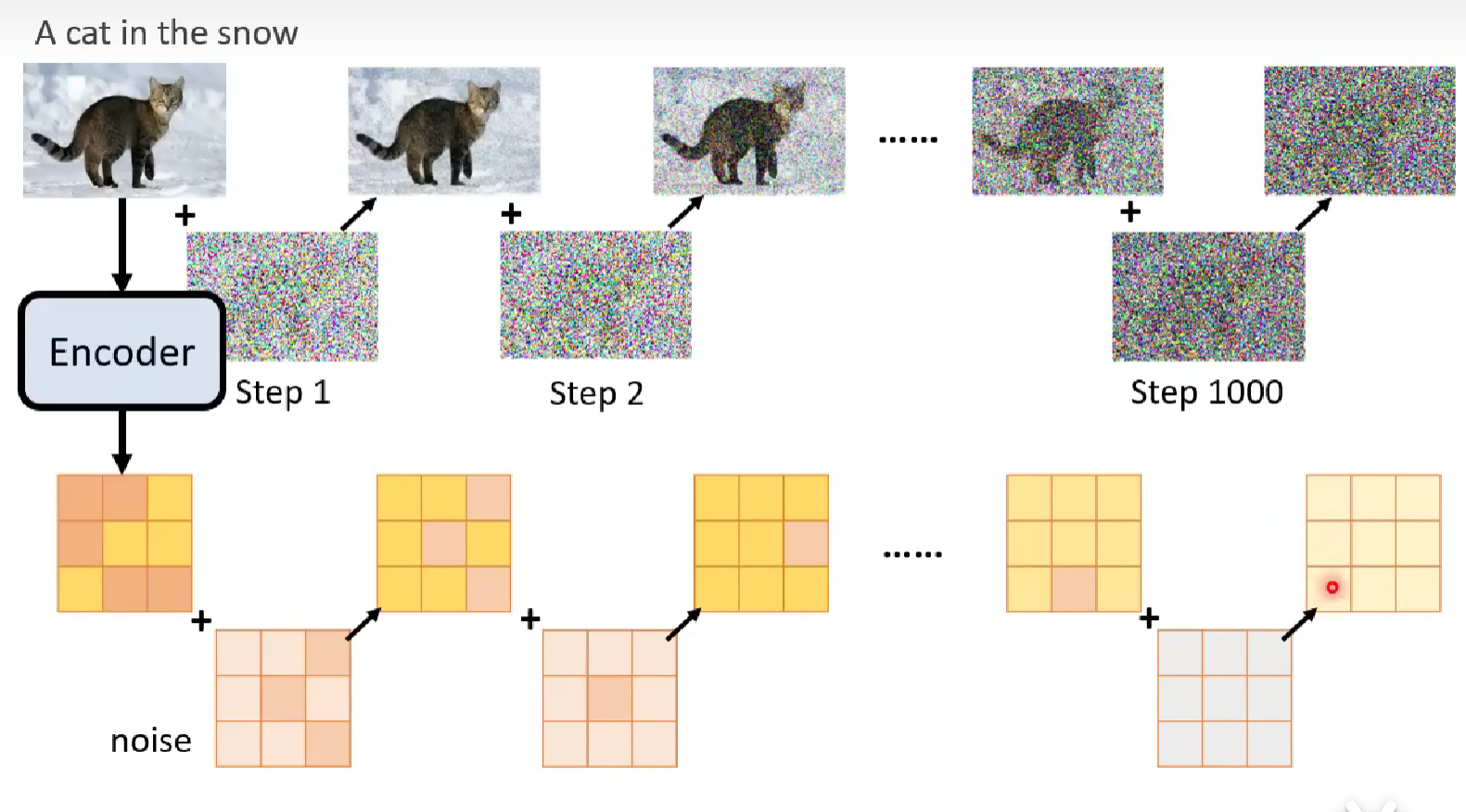
And we train the noise predicter in the following way

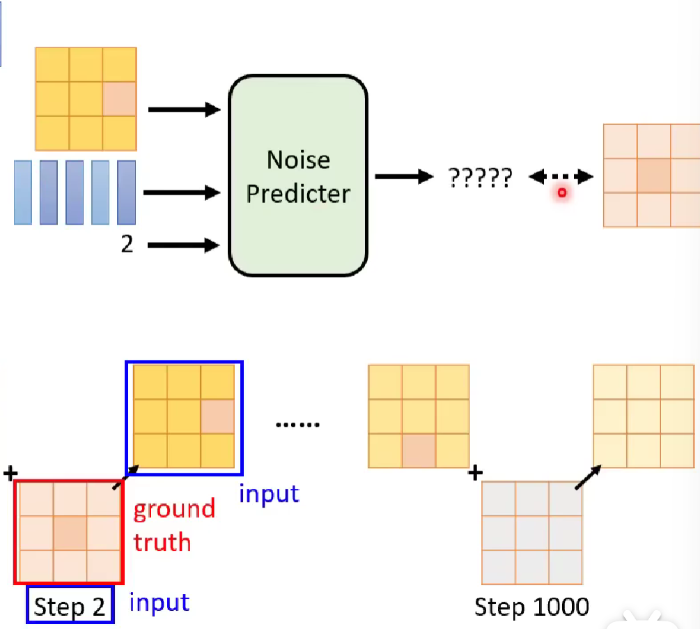
The input is the diffused image (or in same meaning, the previous denoised image), the timestamp and the embedded text prompt. The ground truth is then the noise picture.

Denoise Model

Introduced in previous section, just the noise predicter + subtraction gate.

Denoise Process

The denoise process is then responsible for the generating function of the model.

The generation is done by iteratively input the embedded text prompt and the previous denoised image into the denoise model and then output the current denoised image.

Note that at the beginning step, the input is a total random sample from the normal distribution (the same size as the final generated latent representation). This accounts for why the overall input of the diffusion model is a random gaussian sampling with fixed size and the text prompt.

We will talk about the math principles in the next article.