Diffusion Model (II)
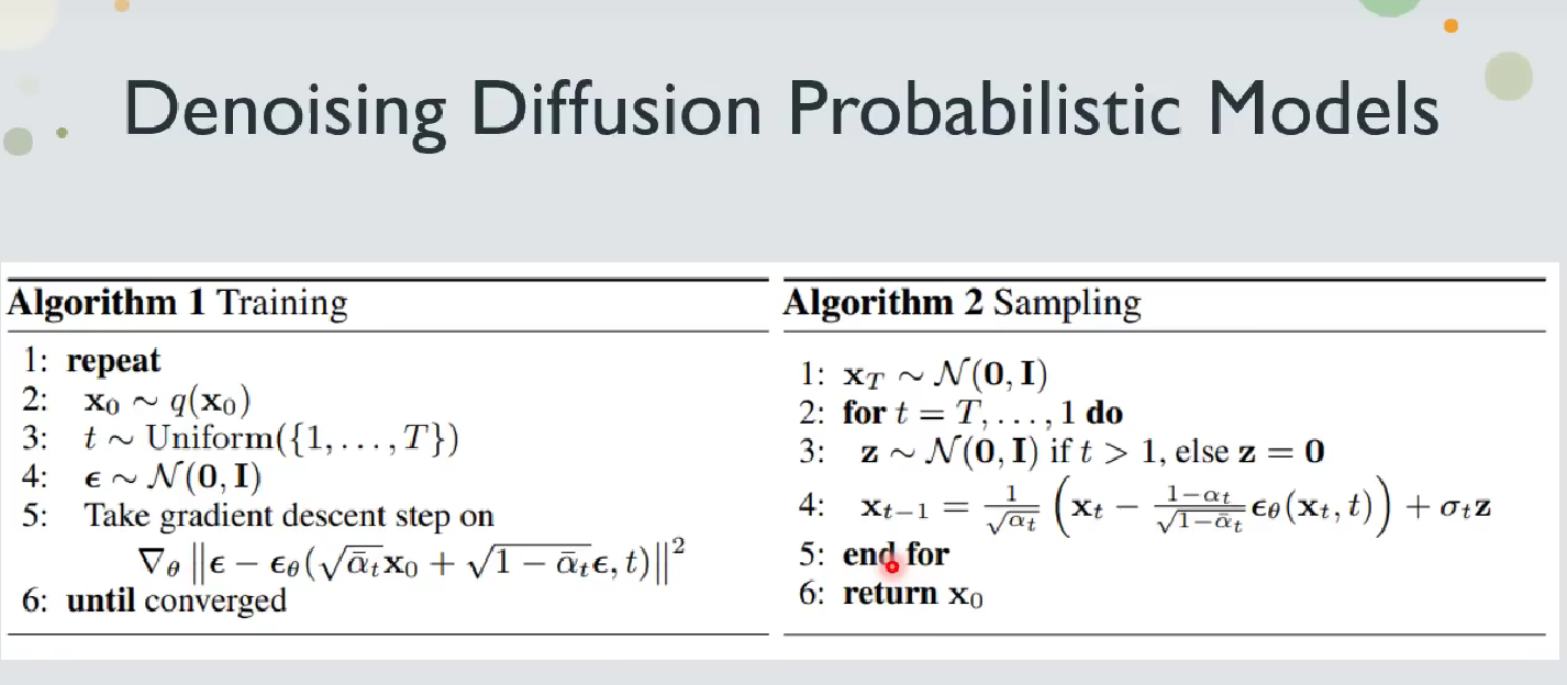
This article is the second part about the diffusion model. In this article, we will show the mathematical principles displayed in the original paper DDPM. We will go through its algorithms, formula deductions and mention several modifications in the realistic model that contrary to our previous layout.
Before we start the deduction part, we first take a look at how the diffusion model is different from the VAE model. Note that we only compare the generative model part of the two model, where their cores lays in.
Now let’s proceed to the algorithm of DDPM
Algorithms
The algorithms of DDPM model can break into two part, the training algorithm and the sampling algorithm (aka the image generating algorithm, which gets its name by starting from sampling on the latent space)
Training Algorithm
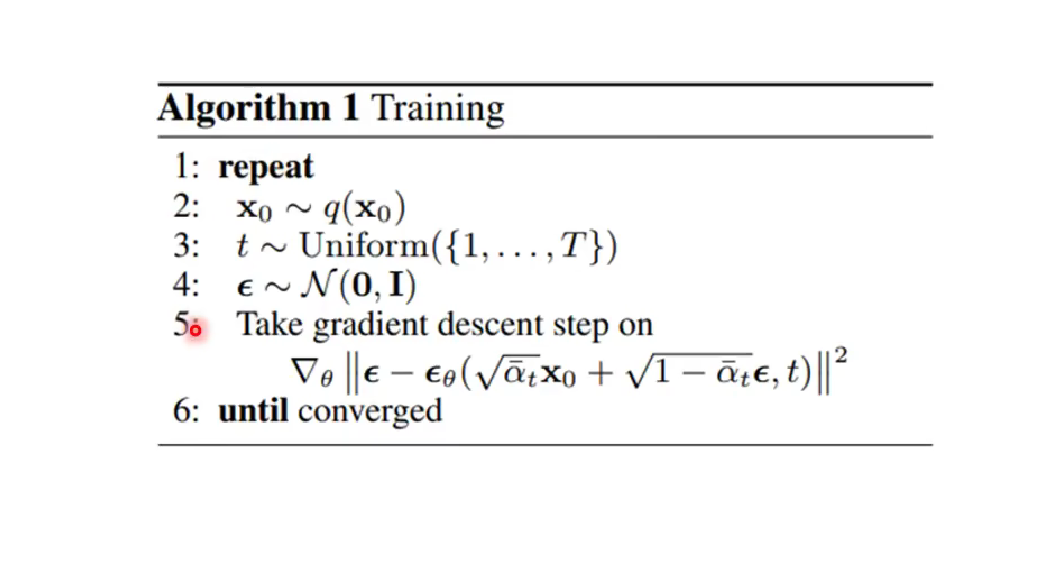
We break the algorithm into pieces.
- Sample a clean image $x_0$ from the image space.
- Sample a timestamp $t$ from 1 to $T$
- Sample an image $\epsilon$ from Gaussian
- Noise the clean image $x_0$ with the noise image $\epsilon$ under weight related to timestamp $t$ (the larger the t, the more noise we exert)
- Send the timestamp $t$ and the noised image to the noise predicter $\epsilon_{\theta}$ , then try to minimize the distance between the predicted noise output and the sampled output $\epsilon$.
- Loop 1-5 until the loss is small enough where we call it to be converged.
This contradicts with our previous view on diffusion model.
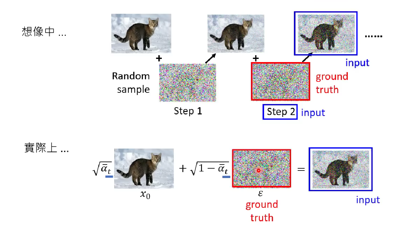
In previous studies, we believe in the diffusion process, the noise is added to or subtracted from the image slowly by each timestamp. And in training the noise predictor, we input the local image and current timestamp and expect a local noise image. Finally we will denoise a photo by iteratively using denoise model step-by-step. (The difference about denoising (or sampling or generating) process will be elaborated in the next section.)
In real DDPM setup, although the amplitude of the noise is still regulated by timestamp. it is added to the image instantly. And in training the noise predictor, the input is the same but we train and expect the output to be the noise image sampled from the original normal distribution.
We will prove it mathematically later.
Sampling Algorithm
The difference about denoising (or sampling or generating) process also is not as drastic as the training process. We first show the algorithm.
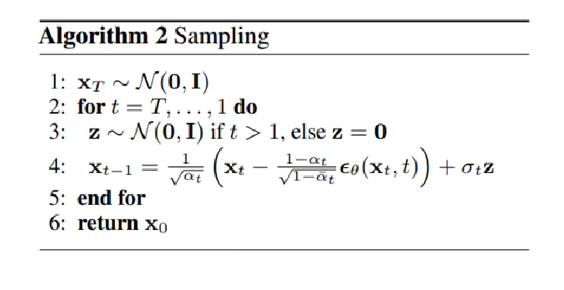
The algorithm is not that different from the previous discussed denoising process, especially in that it also follows the iterative way to denoise, other than that in the training process.
Let’s break it into pieces.
- Sample a complete noise image $x_T$ from the normal distribution
- Loop from timestamp T to 1 to denoise
- Sample another noise image $z$ from the normal distribution $z$
- Input the timestamp $t$ and the previous denoised image $x_t$ into the noise predicter. Output a noise image and let $x_t$ subtract it at a weight related to timestamp $t$.
- Mix the noise $z$ and the output of step 2, the weight is related to timestamp $t$. ( Noise $z$ is zero in the last iteration, namely don’t add noise to the final output).
- Return the final output from the loop. Exit.
A visualized illustration on the denoising process is given below.

Mathematical Principles in Behind
Probability Interpretation of All Generative Models
Before the mathematical formulas, let’s have a look at the probability interpretation on the common goal of every image generative model.
A basic procedure of the image generation model is
- First, randomly sample a vector $z$ from a known distribution (may be simply as unit gaussian). Then feed the vector
- Then, input the vector to a network model, and output another vector $G(z) = x$ . We hope such $x$ is a clean image.
- As we sample more and more different $z$ from the simple distribution, the output samples from the model exhibit (actually follow) a complex distribution. We hope this distribution to be as similar to the real distribution constituted by the real images in the world.
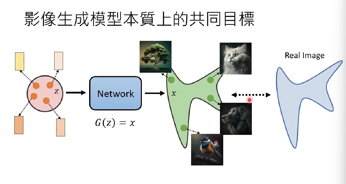
In most applications (like text-to-image model), we should view the output image of the image generative model as a sample from a distribution $p_{\theta}(x|z)$ and we view such distribution as the output of the generative model, giving one input $z$. The else is just the same.
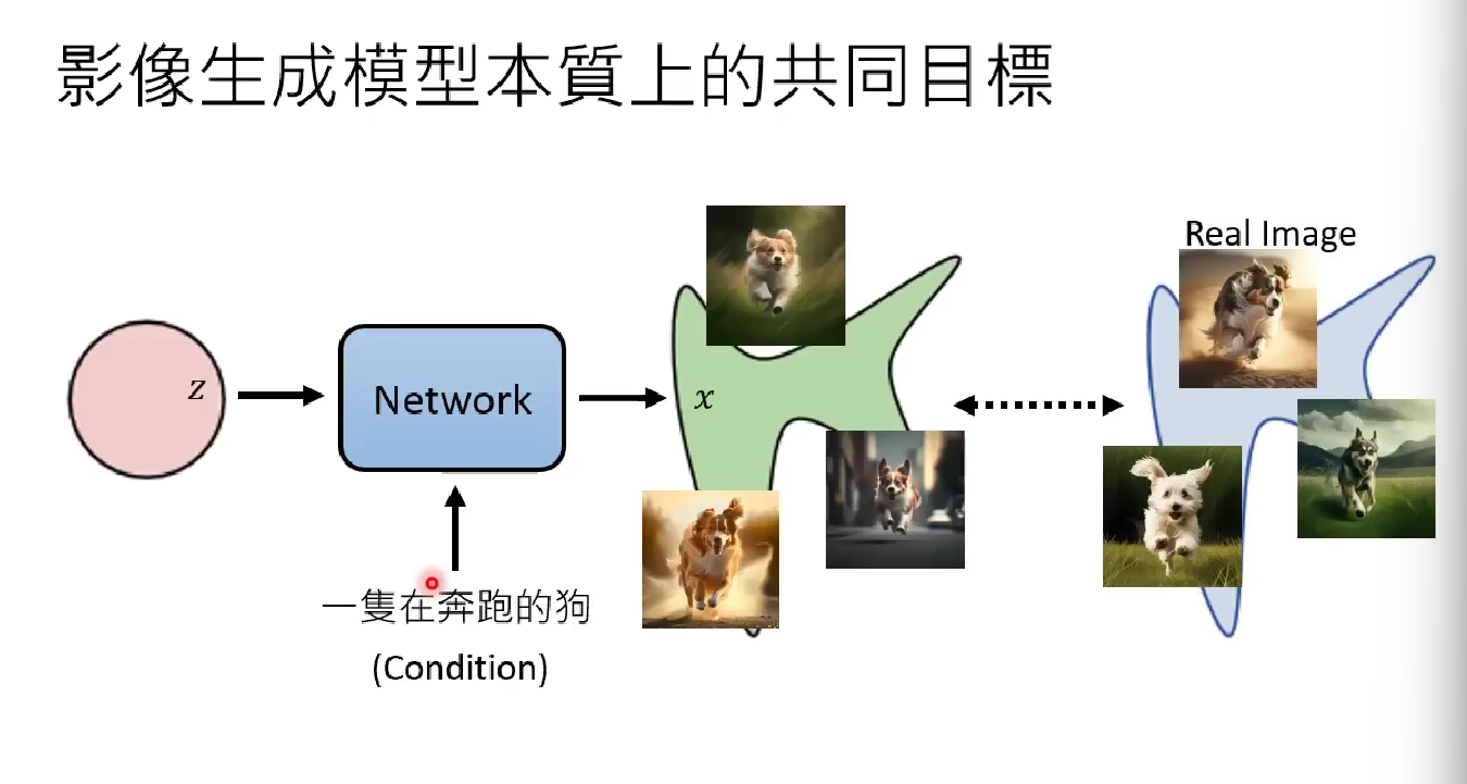
Confusing over whether the model generates a distribution or a vector?
Let’s first tell an example. Normally when we input a text prompt to a language model, it gives different output each time. But we say that the same input vector to the same model will receive the same output vector forever. There seems to be a conflict.
The crux to the conflict is that in real language model, our unchanged prompt does not specify an unchanged input vector $z$. The prompt is directly input as condition to the network model, without interfering the sampling of $z$. Even it does, the prompt still can only specify a range of $z$, not fix it.
So for the question below, it can be a vector or a distribution, like VAE it outputs the parameters of a gaussian distribution, but for the above example the answer should be a vector. Despite this, during the process that the generative model output the vector, it samples $z$ from a simple distribution, which result in the output vector to differ each time, which is actually sampling from a transformed distribution from $z$, controlled by model $G$.
Correctness of VAE Recap
Before we prove the correctness of the diffusion model, we first make an analogy between diffusion model and VAE model. They deal with the generation probability $p(x)$ in the same manner.
There are many connection between the VAE and the diffusion model.
First, their input and output setup are similar. VAE calculate the mean and variance of a unit gaussian distribution as its output. Diffusion model also use a gaussian model as an output, but was generated by denoise.
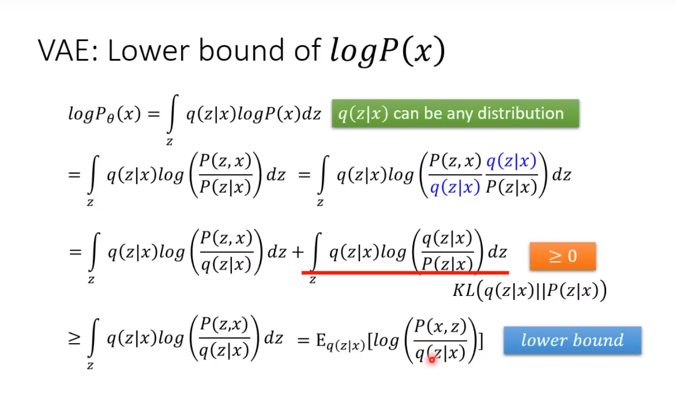
Second, their correctness are similar. We know that VAE wants to maximize the lower bound of the maximum logarithm likelihood function of the model, at the concession that we cannot directly calculate the maximum likelihood function $p_{\theta}$ .
Prove from model’s perspective
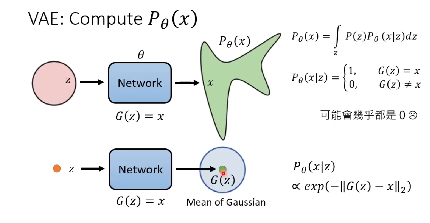
Then how to know from the model’s perspective that we are optimizing $p_{\theta}(x)$ ? We can look at the formula given above.
$$
\begin{aligned}
& P_\theta(x \mid z) \propto \exp \left(-|G(z)-x|_2\right)
\end{aligned}
$$
This formula demonstrate a way to understand why the closer the output $G(z)$ is to the target image $x$, the better the capability of the model can be. Because, the model is trying to narrow the gap between output $G(z)$ and label $x$ , which is the RHS of the formula. Now we say doing this is in proportion to maximize the conditional probability, which is what we want a generative model to do in the previous section. Thus this justifies our VAE model in the model’s perspective.
Proof from Mathematical Perspective
Finally we proof VAE is (indirectly) optimizing $p_{\theta}(x)$ from the mathematical perspective.
Correctness of Diffusion Model
Now we will shift back to Diffusion Model.
DDPM also wants to compute and maximize the MLF $p_{\theta}(x)$. In mathematical level, they are more similar, but in the model’s perspective, we need to bear in mind some differences.
Proof from Model’s Perspective
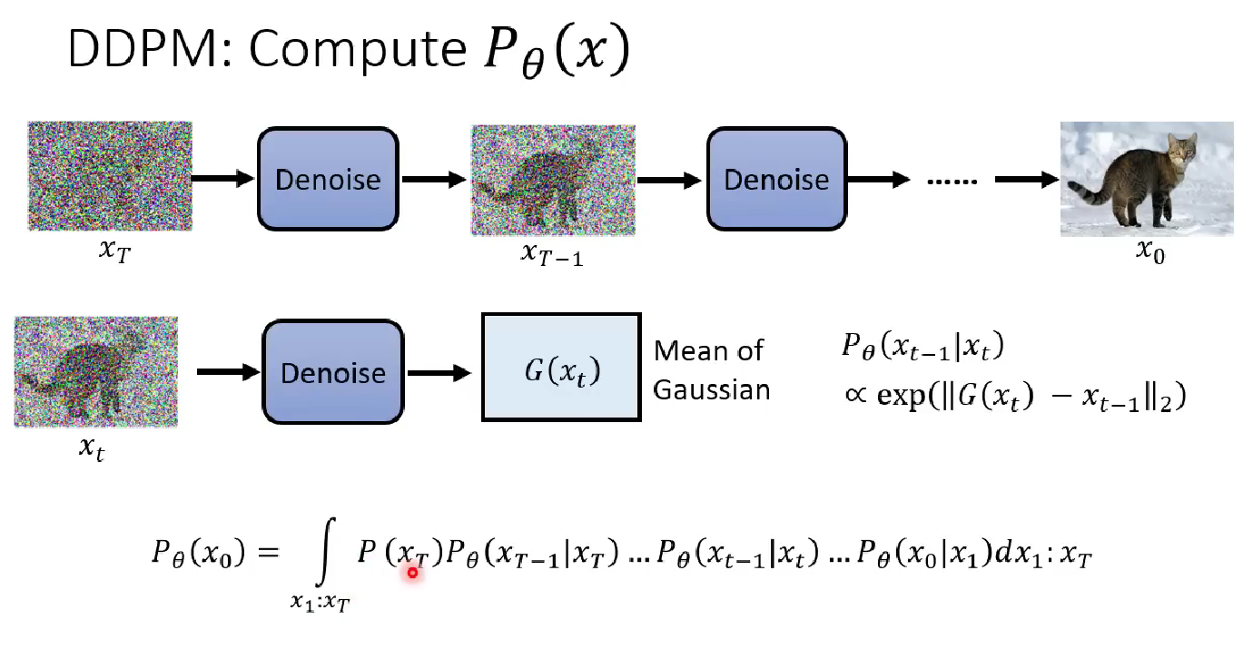
In model level, instead of output the generated image at once, DDPM goes through a sequence of denoising process, each performing independently and contribute to the generated image.
First, we see what each denoising model does at timestamp $t$, is to generate an image $G(x_t)$ that is similar to the label image at timestamp $t-1$, namely $x_{t-1}$.
Then, we can further prove that narrowing the distance between $G(x_t)$ and $x_{t-1}$ contributes to increasing the probability of generating label $x_{t-1}$ conditioned on label $x_t$, namely $P_{\theta}(x_{t-1} | x_t)$ .
Finally, given we want to maximize $p_{\theta}(x_0)$ (the original image before diffusing), we can rewrite its probability using the chain rule of conditional probability. Therefore, we can conclude that what the model is doing helps generating a better image.
Notice that also we can justify the method in such manner, we cannot compute these $p(x_t | x_{t-1})$ conditional probability terms. Labels are not built and calculated by model.
The following illustration echoes the meanings above.
Proof from Mathematical Perspective
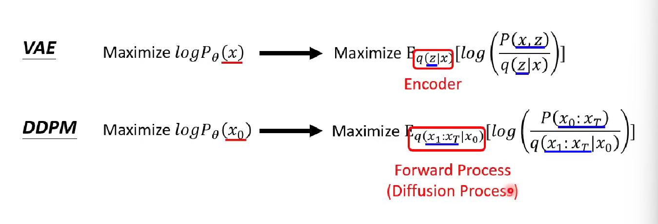
The illustration is a brief of the central idea and captures the similarity of VAE’s and DDPM’s mathematical deduction.
In VAE however, we can directly understand $q(z|x)$ because it is from the encoder’s weight to decide what $z$ to generate given $x$. But in Diffusion Model, it is replaced by a joint distribution representing the diffusion process. Such process requires multiple diffusion steps, making it a bit complex than VAE in analyzation. We need to preprocess and decompose it to parts we can handle. The mathematical deduction steps are shown below.
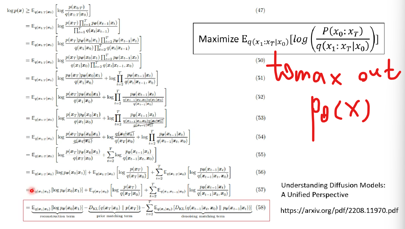
After decomposition, we get three components in the equation. We can match what we’ve computed terms in with this equation.
We will show how to compute the KL divergence term. The others are either similar or easy.
Note: the notation in the diffusion/denoising process is:
1, 2, ..., t, ..., T, ..., t, ..., 2, 1
- Computable: $p_{\theta}(x_{t-1}| x_{t})$ , $p(x_T)$, $q(x_t | x_{0})$
- TBD: probability related to $q(\cdot | \cdot)$
We first explain the computable terms.
To explain the computed terms, the term with $\theta$ subscript is the model’s output, and we can directly evaluate it from the model output. The term $p(x_T)$ is the probability of choosing a sample $x_T$ from the gaussian noise. It is set by us and is thus computable too. The term $q(x_t | x_{0})$ is also computable. Recall $p$ is the probability in denoising process, $q$ is the probability in the diffusion process. We diffuse a image by mixing the original image with a sample of Gaussian noise, with weight related to timestamp $t$. Note that we are not using the previous diffused output $x_{t-1}$ so we haven’t computed $q(x_t | x_{t-1})$ yet.
Let’s see how to compute the TBD terms
First, $q(x_t | x_0)$. That is not hard, because we know $q(x_t | q_{0})$ from diffusion process, and we understand diffusion process from 0 to T can be decomposed into 0,1,…,T. We now have to reversely compute the probability of $q(x_t | x_{t-1})$ that we previously described and assigned in my last blog.
The following illustrate how we deduce from $q(x_t | x_0)$ to $q(x_t| x_{t-1})$ . The last row is $q(x_t| x_{t-1})$, the row above are several diffusion steps in our model (starting from $x_0$).
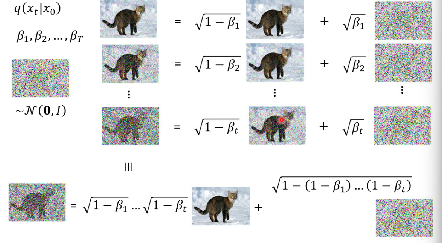
Thus we conclude $q(x_t | x_0)$ is computable.
Second we will compute $q(x_{t-1} | x_t, x_0) $. We can already compute the following terms:
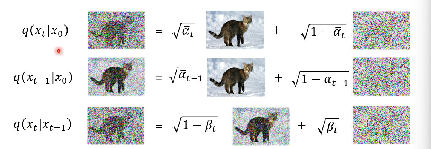
Here is how we use the above to deduce our goal.

The concrete deduction (from normal distribution) is given below.
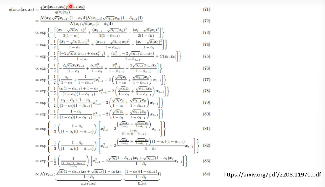
After reduction, we find $q(x_{t-1} | x_t, x_0)$ is still a gaussian distribution, and the mean and variance of this distribution is given below

Finally, we compute the KL Divergence.
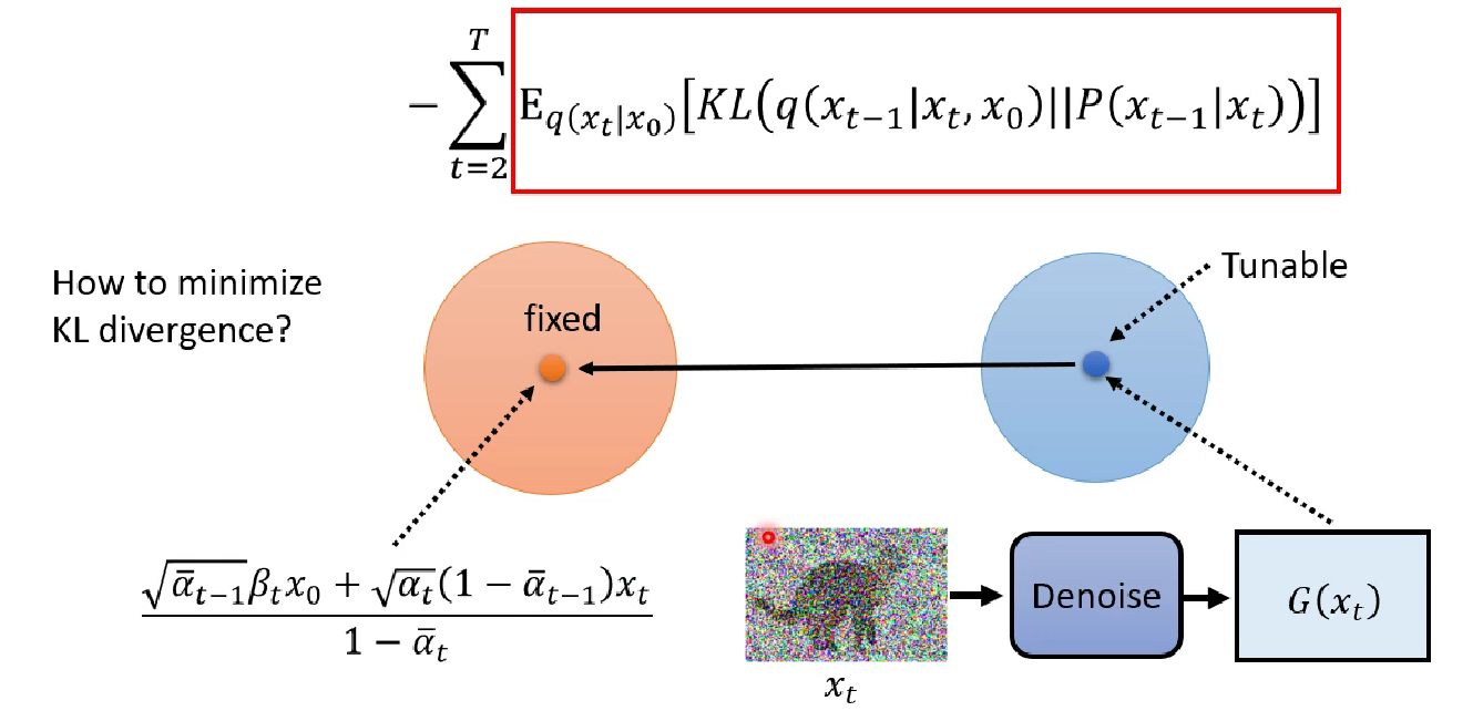
From the network training perspective. We want the KL distance to be as small as possible. The orange circle is the distribution of $q(x_{t-1} | x_t, x_0)$ , and the blue is the distribution of $P(x_{t-1} | x_t)$, which is the output of our model. By our assumption, he blue circle has fixed variance and tunable mean from the model, so we only need to move the mean of the blue circle close to orange distribution model as much as possible.
Final Step
Now the logic is as below, if we want to prove from mathematical perspective, we need to convince ourselves that the model is optimizing the $p_{\theta}$ and in other words, the model is optimizing the KL divergence and by our deduction before, the model is trying to narrow the gap between the mean of model output and the computed mean of distribution $q(x_{t-1} | x_t, x_0)$.
We now prove it is indeed the truth.
What our model does in training and sampling is respectively

and

The first formula in the paper is the same as ours in generating $x_t$ in diffusion process.
The second formula in the paper is the same as ours in denoising and generating $x_{t-1}$. The deduction is given below
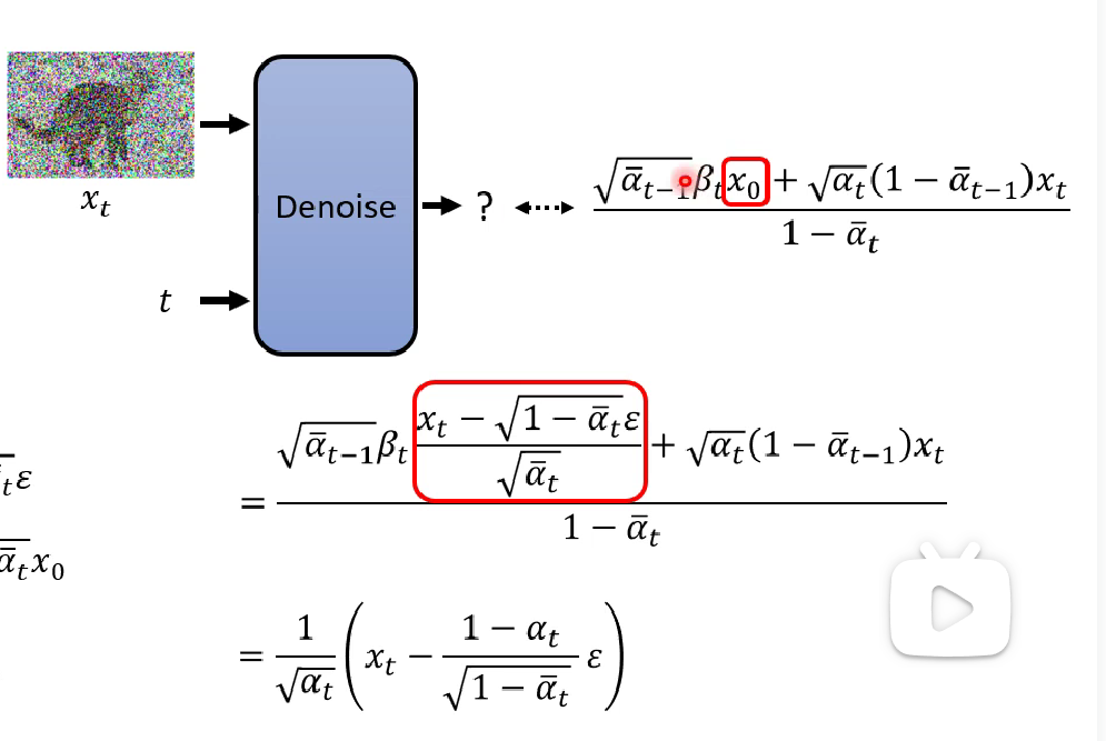
Thus we justified that the paper’s method is indeed training model to generate a better image.


